Overview

For this assignment, I implement an array of basic geometry processing algorithms and techniques to render realistic-looking 3D meshes on the screen. Section I covers drawing and shading of Bezier surfaces, which are conceptually simpler to grasp but more difficult to render in real life than triangle meshes, which are explored in Section II. Although the Half-edge data structure has many components that took me a while to grasp initially (and requires careful tracking of many variables and pointers, which made for some fun debugging and typo-catching), I also now believe that it is very powerful and useful, as can be seen in Part 6 of this assignment, where a coarse mesh can quickly be upsampled into a very high-resolution rendering.

Section I: Bezier Curves and Surfaces

Part 1: Bezier Curves with 1D de Casteljau Subdivision

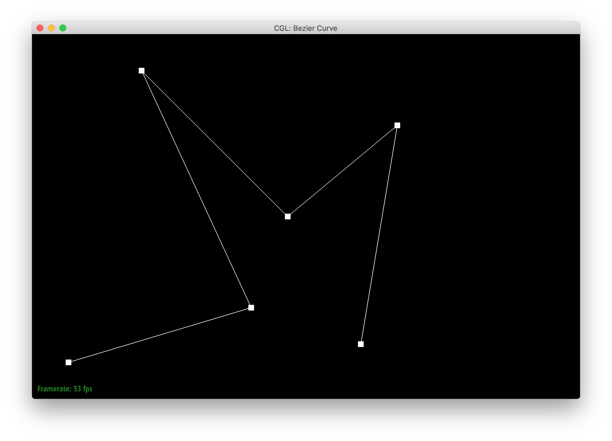
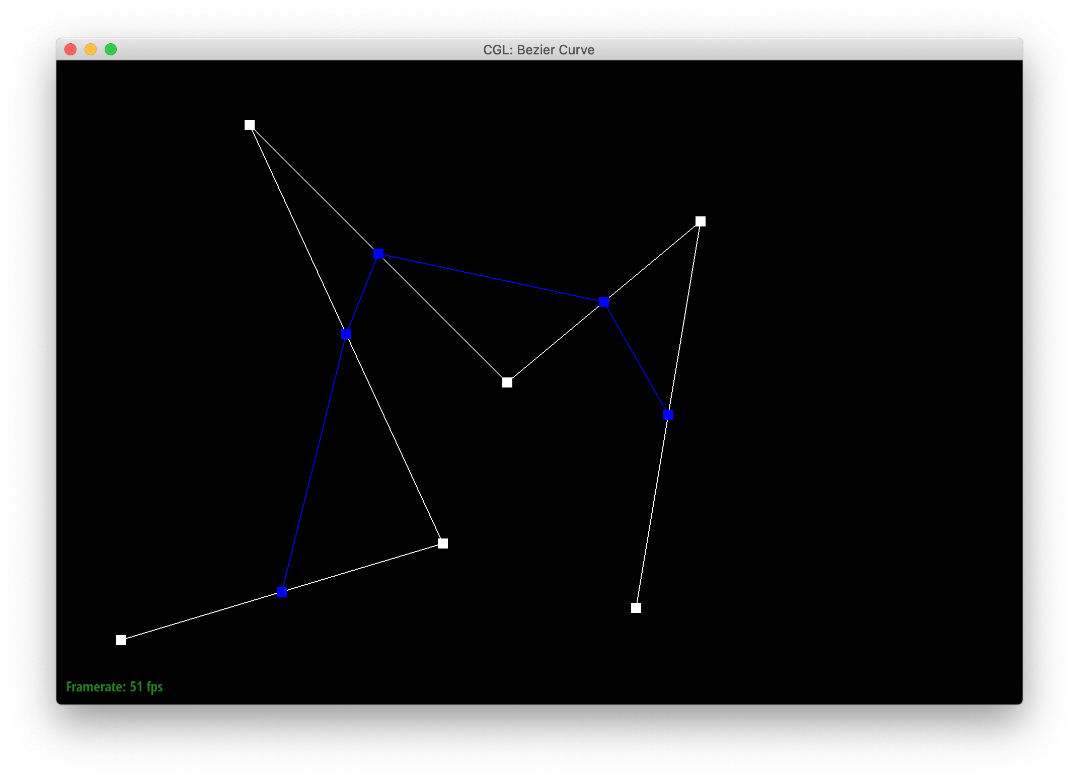
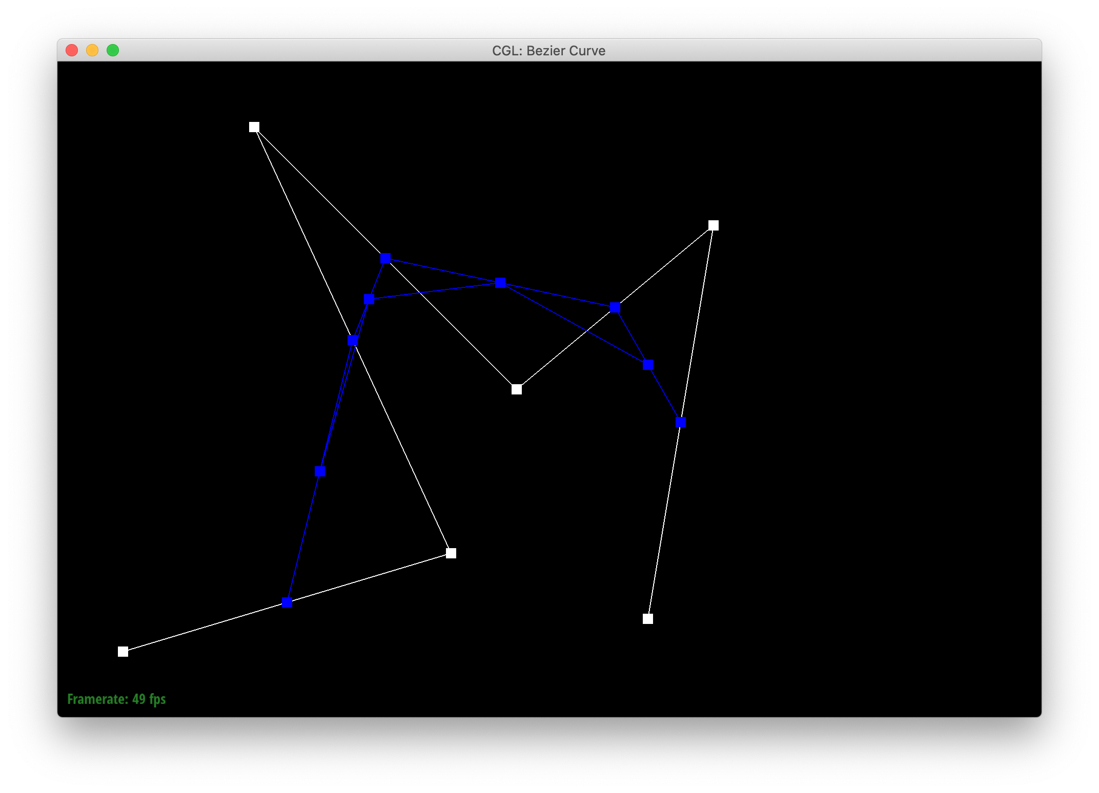
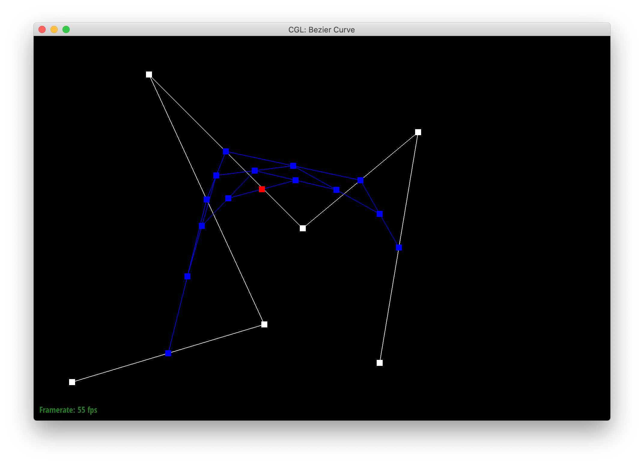
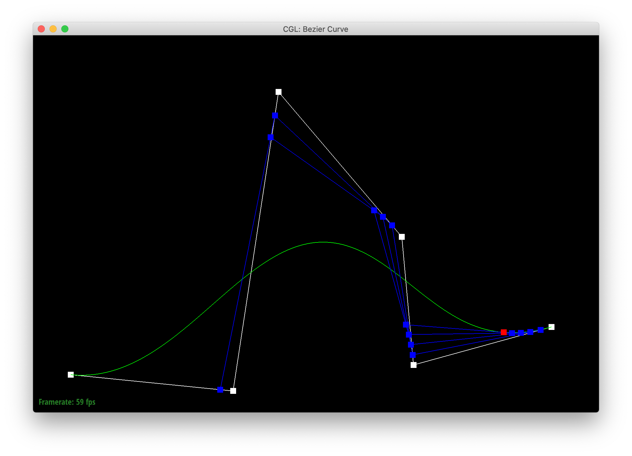
de Casteljau's algorithm is a recursive method of evaluating a Bézier curve given a set of n control points and parameter t. The algorithm starts by defining a set of intermediate control points to be equal to the original control points. In each step, if there is still more than 1 intermediate control point remaining, a new set of intermediate control points is constructed by linearly interpolating between each pair of adjacent intermediate control points with the parameter t. This results in the number of intermediate control points reducing by 1 in each step. Eventually, there is only 1 control point remaining, and this corresponds to the point on the Bézier curve at parameter t. The entire Bézier curve may be constructed by repeating this process for all t. In Part 1, I implemented 1 step of de Casteljau's algorithm in the evaluateStep function by creating a std::vector<Vector2D> array of intermediate control points. For every given control point except the last one, I add a new control point to this intermediate control points array that is the linear interpolation of that control point plus its following neighbor.

Below are screenshots of each step of the evaluation from 6 original control points down to the final evaluated point on my curve, my_curve.bzc.

Below is a screenshot showing the completed Bezier curve:

Below are screenshots showing a resulting Bezier point/curve after moving the control points around and varying t:

Part 2: Bezier Surfaces with Separable 1D de Casteljau

A Bezier surface may be thought of as being generated by an n x m array of control points instead of an n-length list of them. de Casteljau's algorithm may thus be extended to generating Bezier surfaces by first running the algorithm along one dimension given the parameter u - which results in a list of control points along the second dimension, and then using that list as input for de Casteljau's algorithm along the second dimension given a second parameter v to find the point that lies on the Bezier surface at the parametrization (u,v). The entire Bezier surface may then be generated by evaluating along all valid u and v, just as a Bezier curve is generated by evaluating the algorithm for all t.

The evaluateStep function that evaluates a single step of de Casteljau's algorithm is the same as that in part 1 except for the fact that the input and return arguments are of the std::vector<Vector3D> type instead of the std::vector<Vector2D> type. This function is called recursively by the evaluate1D function until the single, final interpolated vector is left. In the evaluate function, a list of intermediate control vectors is created. For each control point in the x dimension, evaluate1D is called with the parameter u, and the result is added to the list of intermediate control vectors. evaluate1D is then called upon the final list of intermediate control vectors given the parameter v to find the point at (u,v) that lies on the Bezier surface.

Below is a screenshot of bez/teapot.bez:

Section II: Triangle Meshes and Half-Edge Data Structure

Part 3: Area-Weighted Vertex Normals

I implemented area-weighted normals in the Vertex::normal() function. I start by defining the halfedge associated with the current vertex and initializing an empty to-be-normalized normal vector. I then set up a do-while loop, using the printNeighborPositions function in the Halfedge primer document as a base to handle boundary cases. Within the do loop, if the face associate with the current halfedge is not a boundary face, I find the vertices of the face associated with the current halfedge with the halfedge's next() and next()->next() functions, and I take a cross product between the 2 vectors spanning between consecutive vertices. This cross product, whose norm is twice the area of the triangle, is added to the running normal vector. Since this vector is normalized in the end, we do not have to be concerned with the fact that we're technically calculating 2 times the area of each triangle. The loop then moves on to the next vertex using the halfedge's twin()->next() functions, and if we haven't returned to the original halfedge, the loop continues. When the loop terminates, the normal vector is normalized and returned.

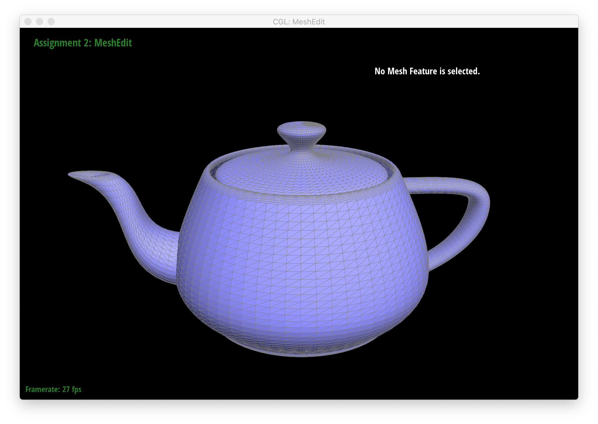
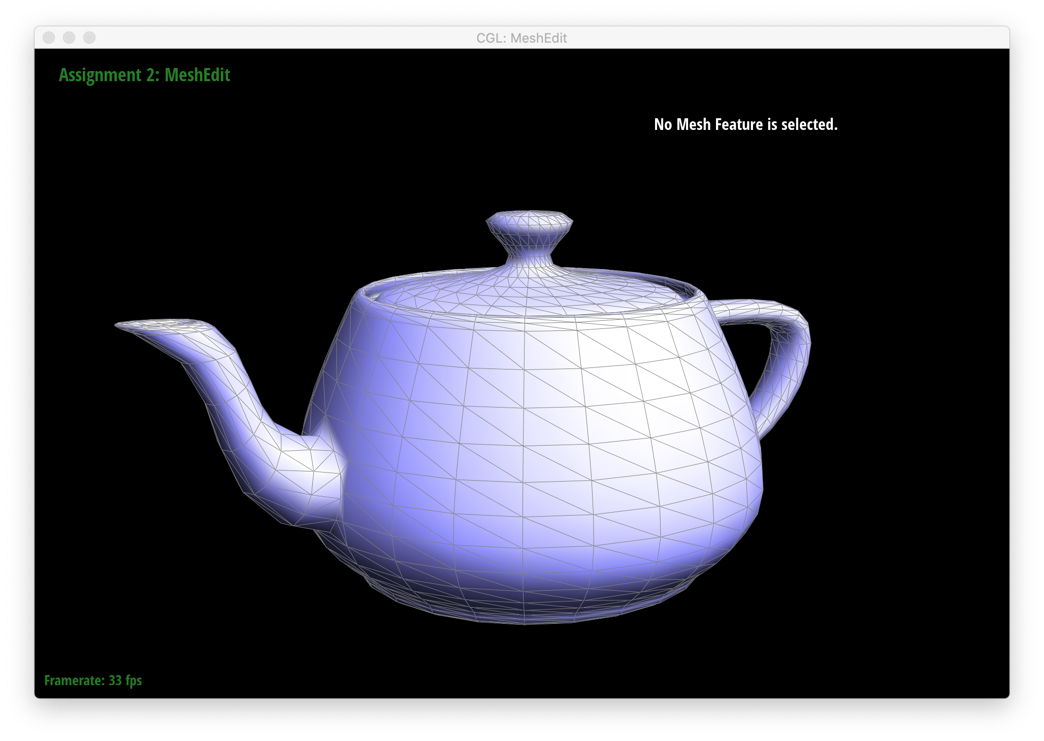
Below are screenshots showing teapot.dae before and after using area-weighted normals for shading.

As clearly seen above, shading with area-weighted normals yields far smoother, more "natural" shading than simply coloring each triangle in the mesh with a flat color.

Part 4: Edge Flip

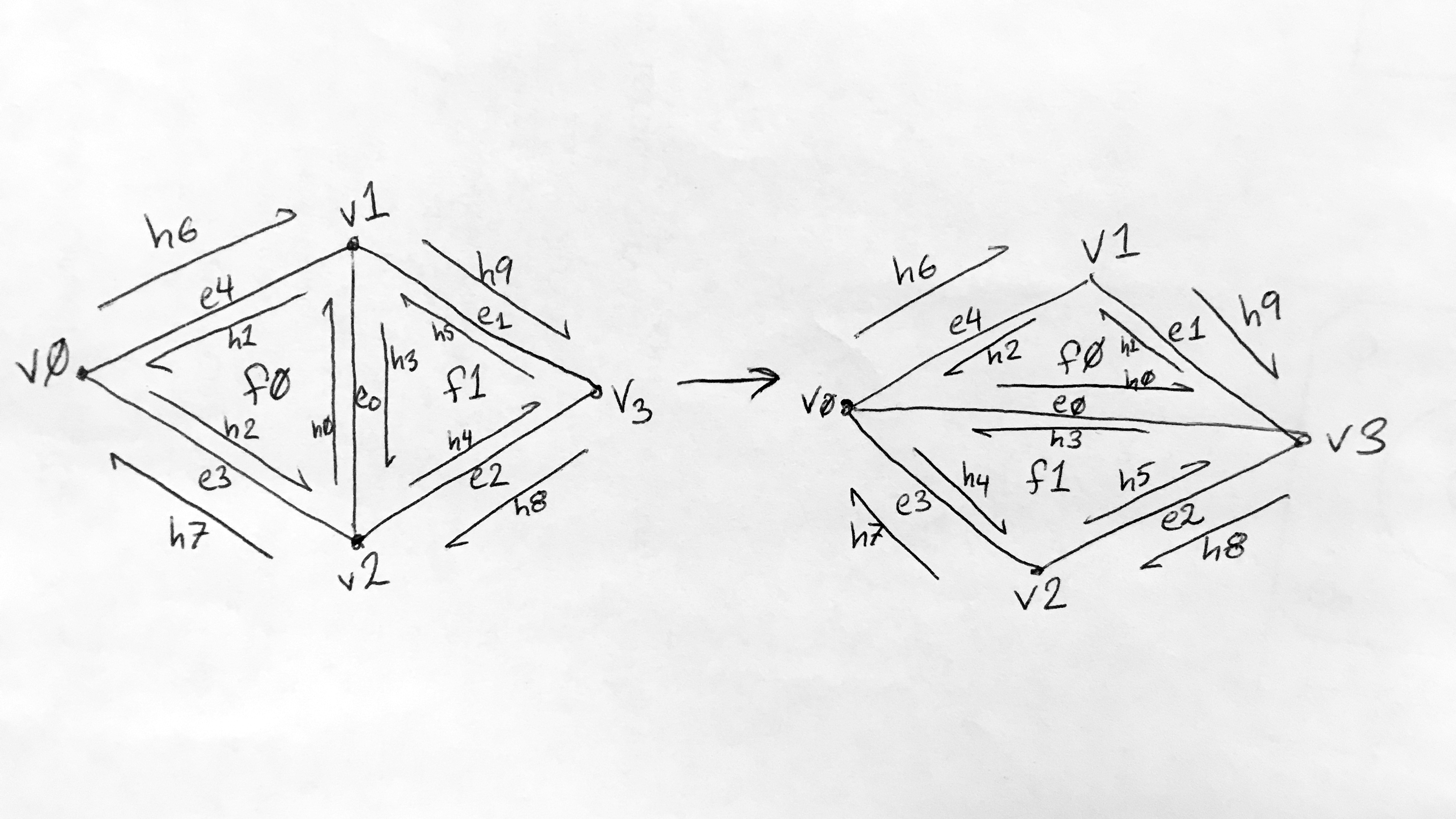
Using the supplemental notes in the Halfedge primer as a starting point, I labeled all halfedges, vertices, edges, and faces associated with the edge flip operation, as shown below:

I then assigned an iterator to each halfedge, vertex, edge, and face based on above left diagram. I then updated each iterator (first the halfedges, then the vertices, then the edges, and finally the faces) based on the post-edge flip diagram, shown on the right above. For the halfedges, I used the setNeighbors function to define each halfedge's new (sometimes unchanged) next, twin, vertex, edge, and face. For the vertices, edges, and faces, I updated those iterators' halfedge() to be the appropriate new halfedge.

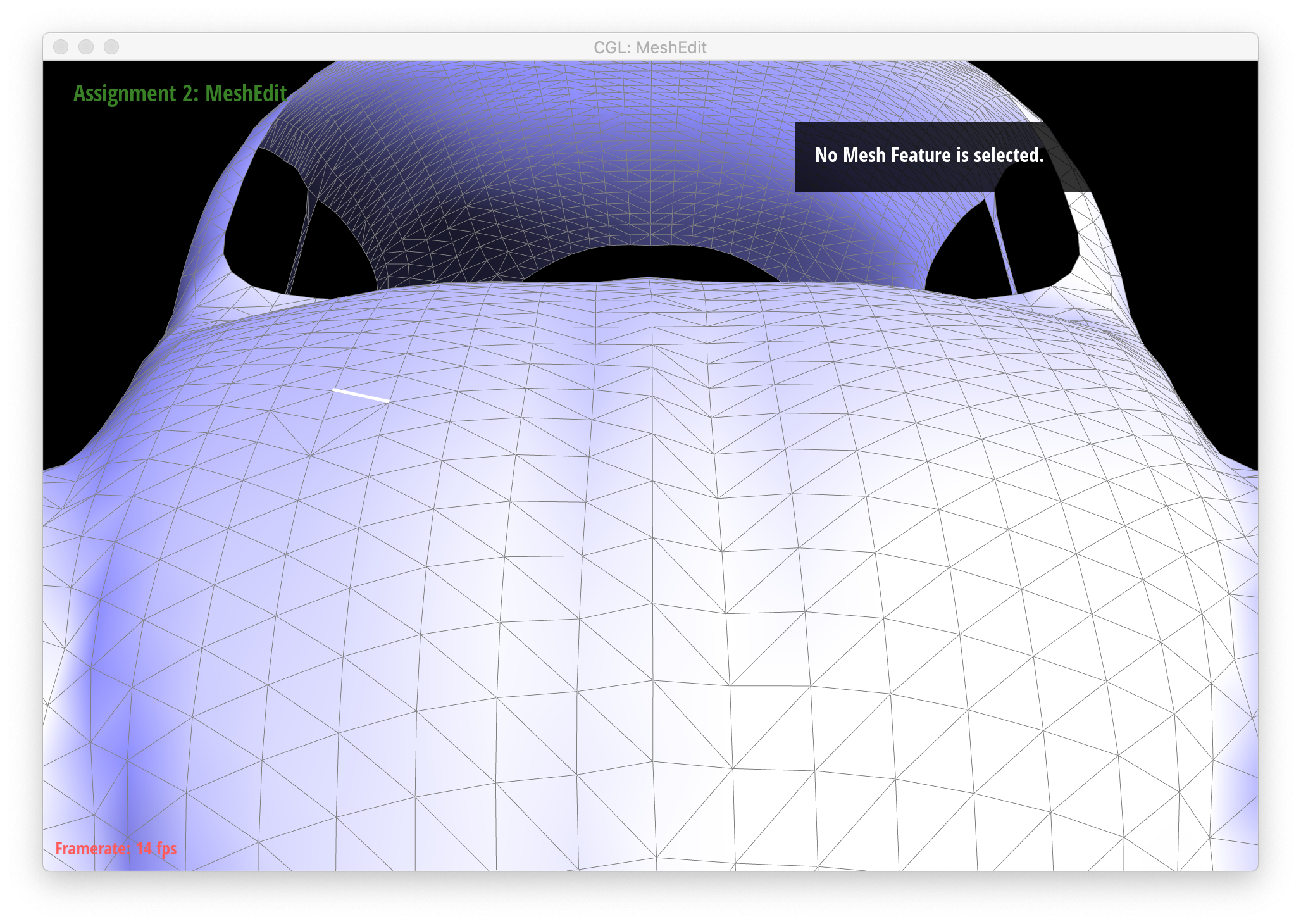
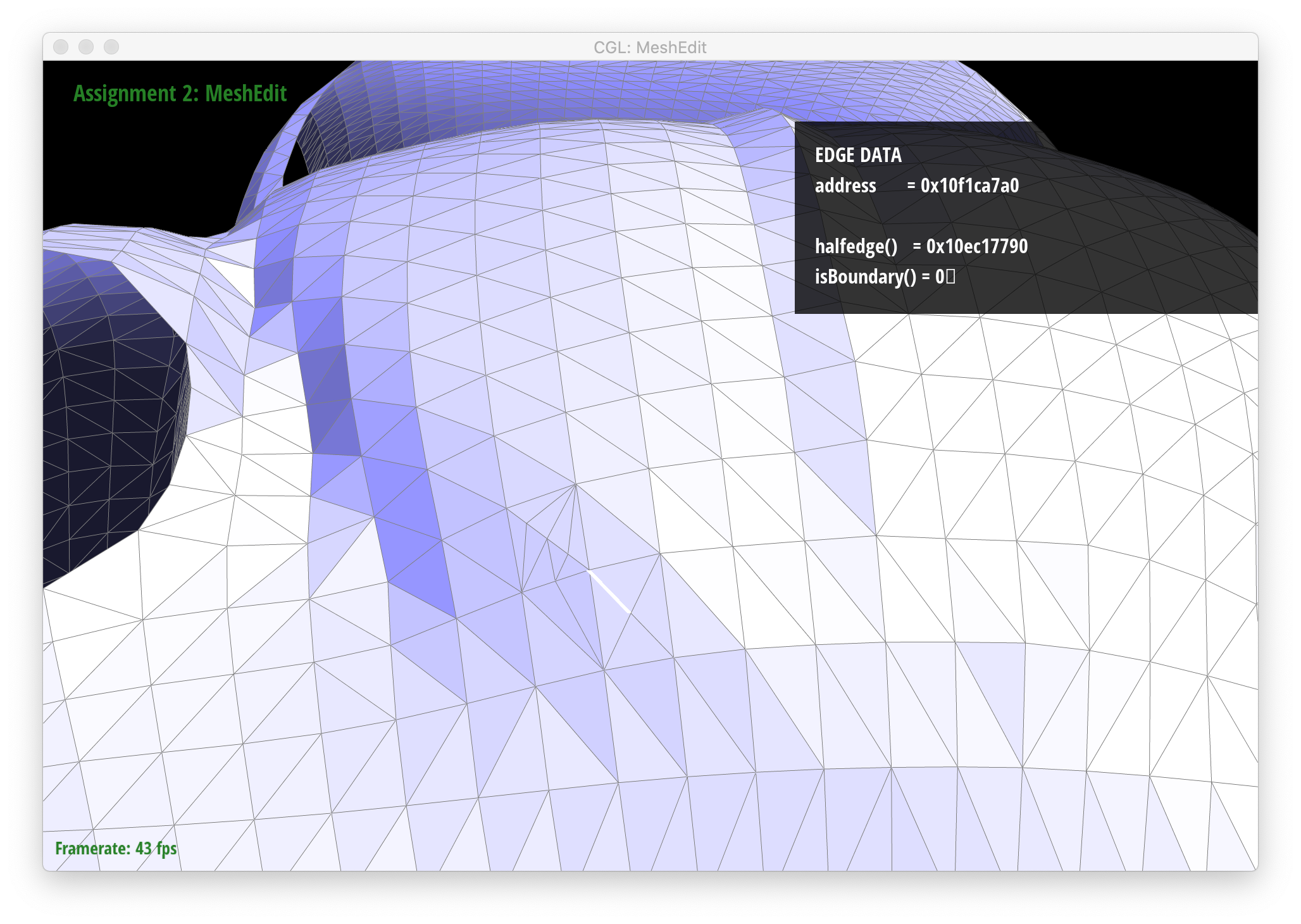
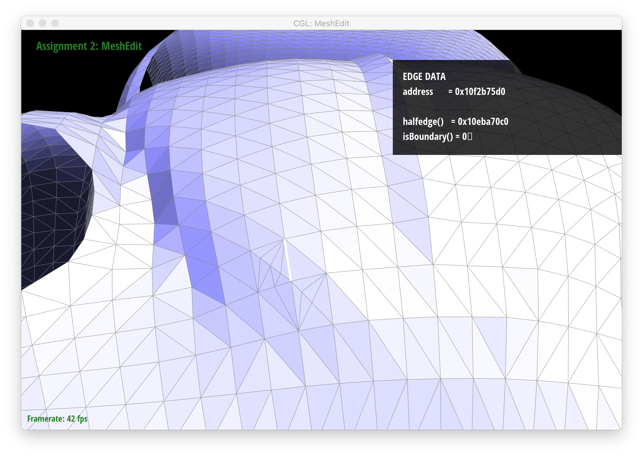
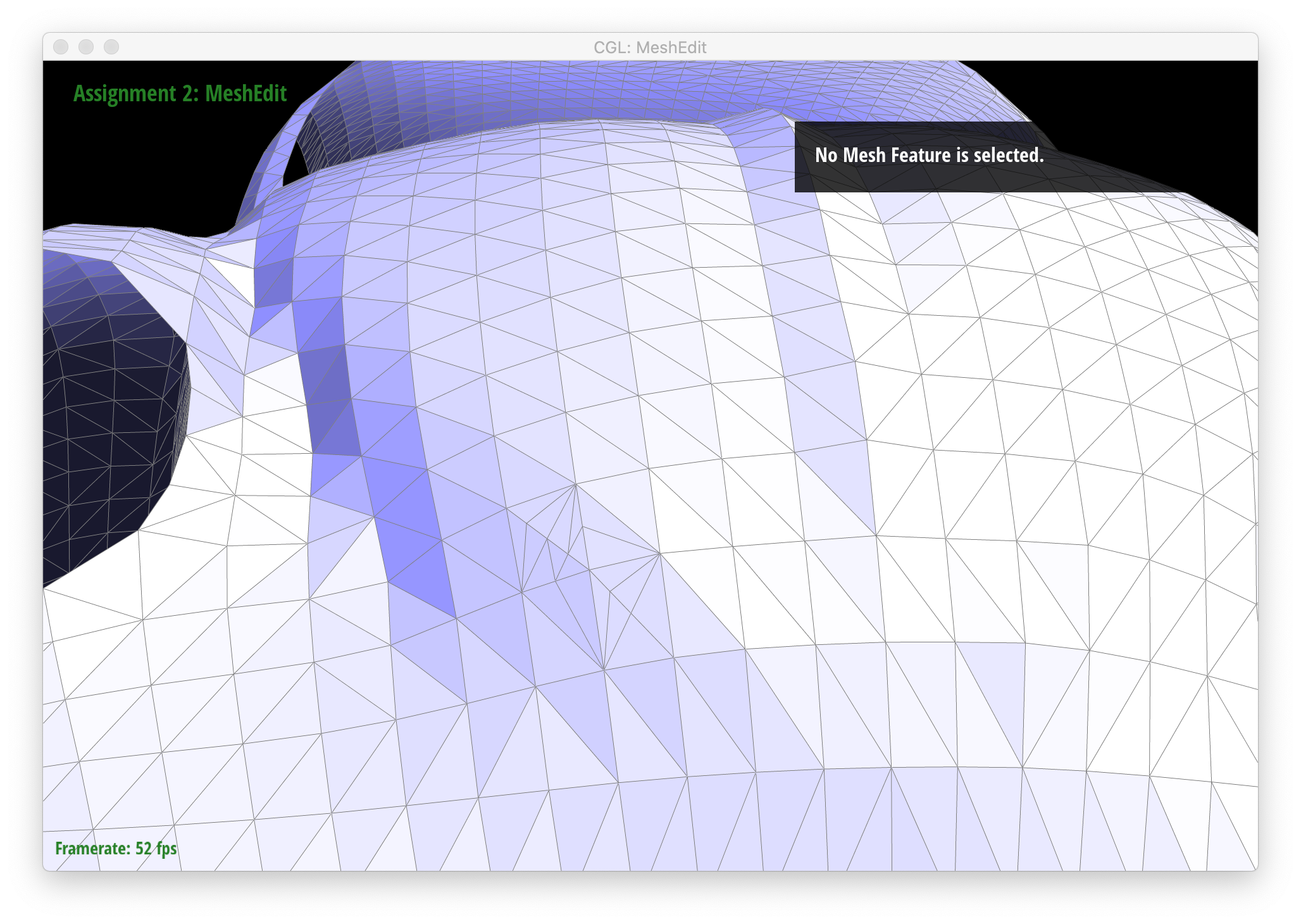
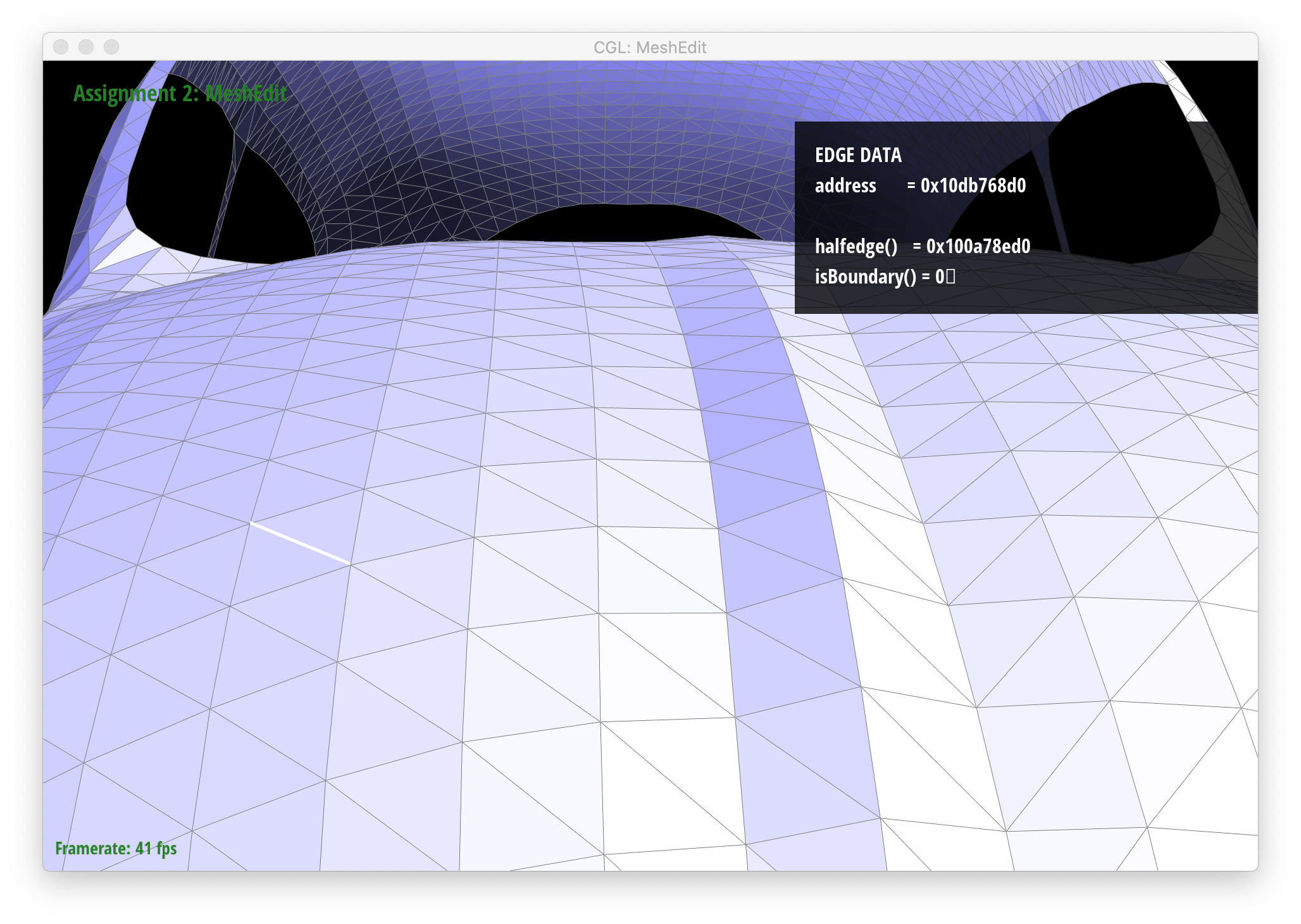
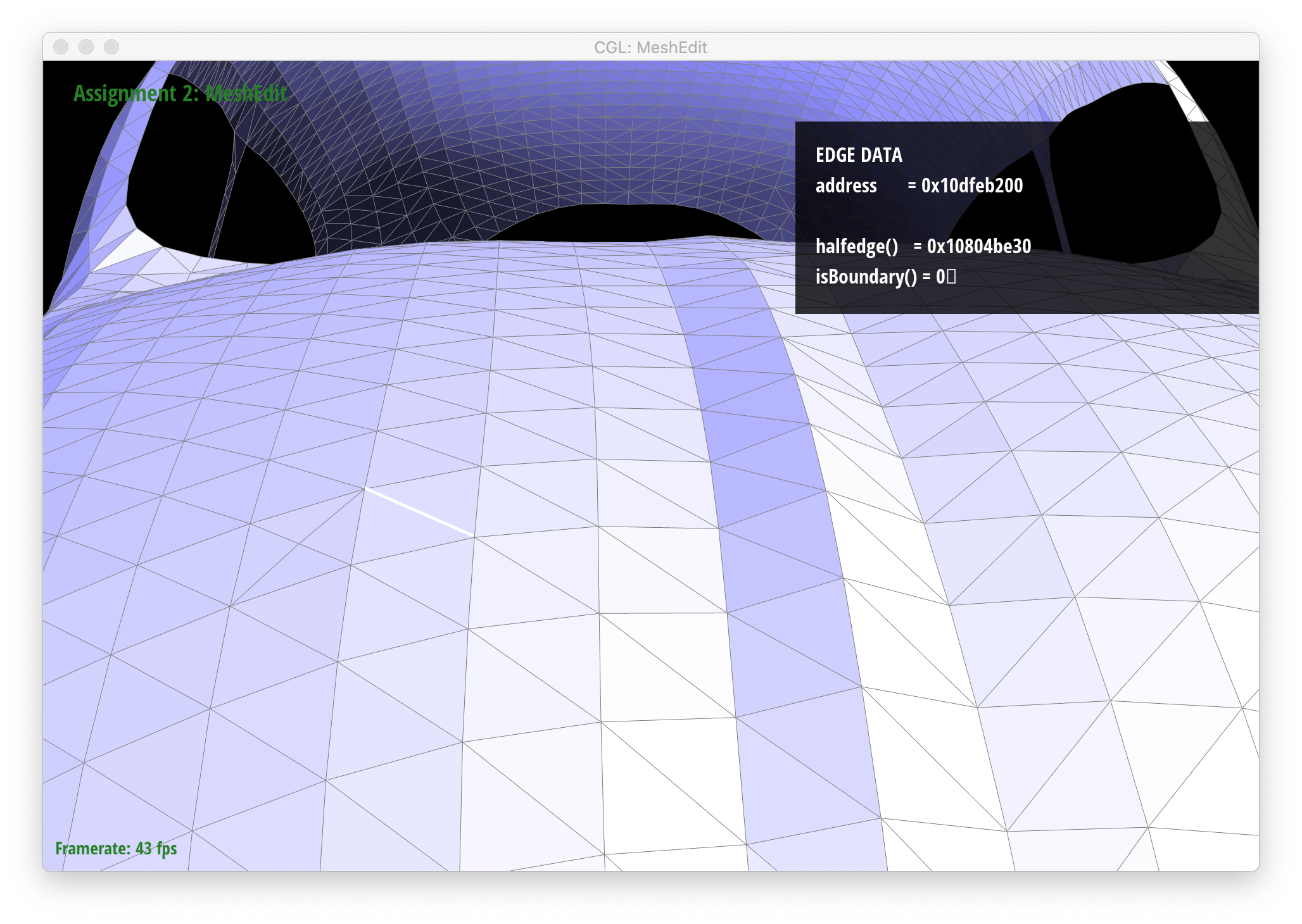
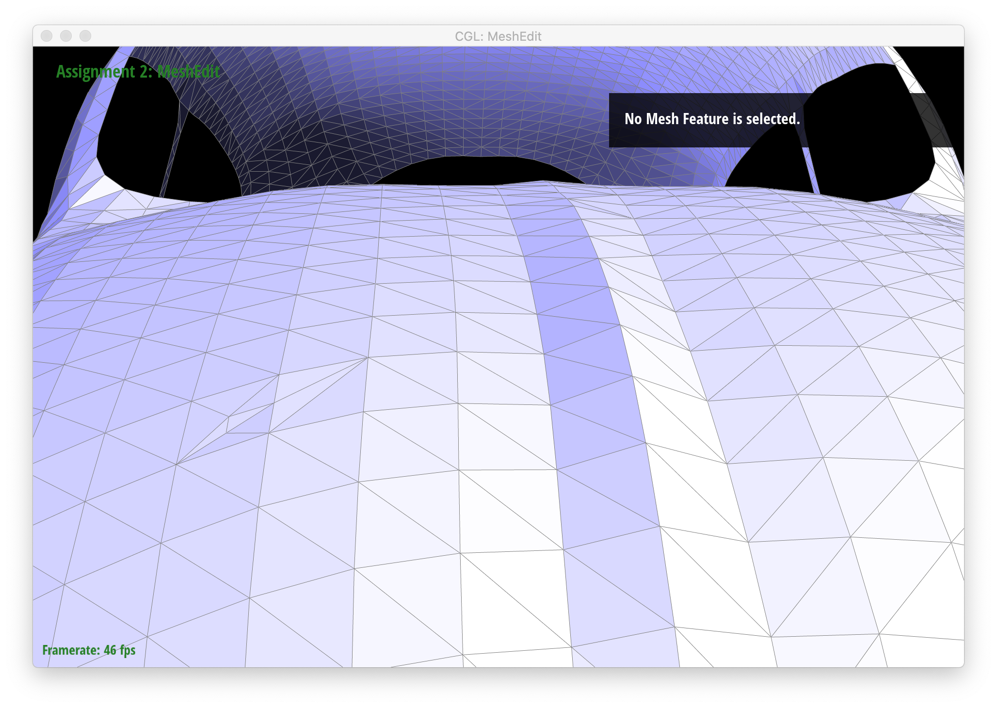
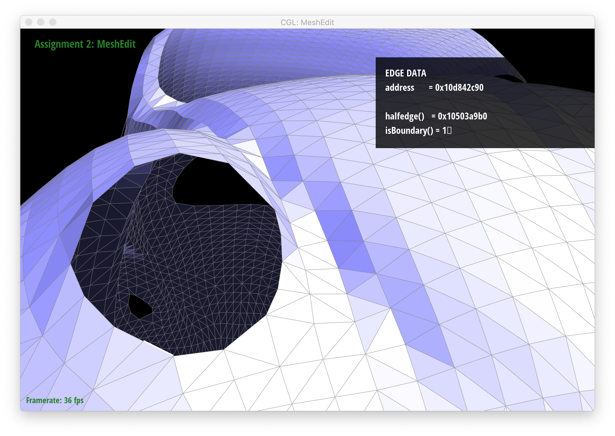
Below is a set of example edge flips (done on beetle.dae using area-weighted normals for shading from Part 3). In each screenshot, the edge to be flipped is highlighted in white.

While debugging, I caught several plain typos in my code, such as assigning a pointer to h0 instead of h5 (don't copy-paste while multi-tasking?). That resulted in mostly correct behavior, but once in a while there were pretty odd errors, such as neighboring triangles disappearing completely. I was also confused at first about which halfedge to assign a given face, vertex, or edge when there was more than 1 option, but upon examining the code, I realized it didn't actually matter.

Part 5: Edge Split

As in Part 4, I labeled all halfedges, vertices, edges, and faces associated with the edge split operation, as shown below:

I then assigned an iterator to each halfedge, vertex, edge, and face based on above left diagram. I then updated each iterator (first the halfedges, then the vertices, then the edges, and finally the faces) based on the post-edge split diagram, shown on the right above. For the halfedges, I used the setNeighbors function to define each halfedge's new (sometimes unchanged) next, twin, vertex, edge, and face. For the vertices, edges, and faces, I updated those iterators' halfedge() to be the appropriate new halfedge. This "trick" helped me make sure that I was keeping track of all elements before and after the split operation

Below are screenshots of a mesh before and after some edge splits:

Below are screenshots of a mesh before and after a combination of edge splits and edge flips:

Again, while debugging, my biggest problem was finding typos. Thanks to my messy handwriting and refusal to put my diagram in Illustrator/other similar digital format, I mixed up things like "5" and "15" several times, which would result in mostly-correct edge splits with the occasional odd, wrong behavior. I didn't actually catch some of these until part 6, when I started seeing that splitting certain edges would cause incorrect splits.

Part 5: Extra Credit

I implemented the extra credit to support edge splits for boundary meshes. Similar to my approach for Parts 4 and 5 of this assignment, I created a labeled diagram of a boundary split that I used to keep track of all the Halfedge mesh elements (some of these turned out to be unnecessary/redundant, but I drew them anyway for my own sanity):

Below are screenshots showing proper behavior for boundary splits.

Part 6: Loop Subdivision for Mesh Upsampling

I followed the recommendation in the assignment description to implement loop subdivision for mesh upsampling. More specifically, I first iterated through all halfedges in the original mesh and marked all edges and vertices as old (setting their isNew variable to false). In the same loop, I also pre-computed the newPosition of every vertex and edge. For existing vertices, I used the formula of newPosition = (1 - n * u) * original_position + u * original_neighbor_position_sum, where n is conveniently obtained with the degree() function of the Vertex class, u is assigned to 3/16 for n=3 and 3/(8n) otherwise, original_position is simply the position variable of the vertex, and original_neighbor_position_sum is calculated by traversing the half edges connected to the given vertex and summing up their vertex positions (similar to what was done to traverse halfedges to calculate area-weighted normals in Part 3). For existing edges, I calculated newPosition as 3/8 * (A + B) + 1/8 * (C + D), where A and B are the positions of that halfedge's vertex and its twin's vertex, and C and D are the positions of the halfedge's next()->next() vertex and its twin's next()->next() vertex.

Next, I split every original edge of the mesh. To do this, I modified my splitEdge function from Part 5 to correctly flag the isNew variable of the new Vertex and the new Edge as true (making sure to mark the 2 edges that lie along the original edge as not new). I avoid infinitely looping through edges by capping the number of iterations to the number of original edges and only advancing my loop counter if a NOT isNew edge is encountered and then split. The resulting vertex is flagged as new, and its newPosition variable is updated to be the newPosition of that split edge.

Next, I loop through all edges (including new ones), and any new edge that connects an old and new vertex (i.e. its vertex is new and its twin's vertex is old, or vice-versa is flipped.

Finally, I loop through all vertices (including new ones), and its position is set to its newPosition variable.

I debugged this loop-by-loop, first visually checking that I was correctly splitting every original edge (I found a bug in my original Part 5 code when I did this), then adding the loop where I flip edges, and then finally adding the loop to update all vertex positions. With this method, I was quickly able to realize and fix the fact that I was inappropriately assuming dividing one int by another would result in a double, which in turn resulted in some pretty exciting and wrong vertex position updates.

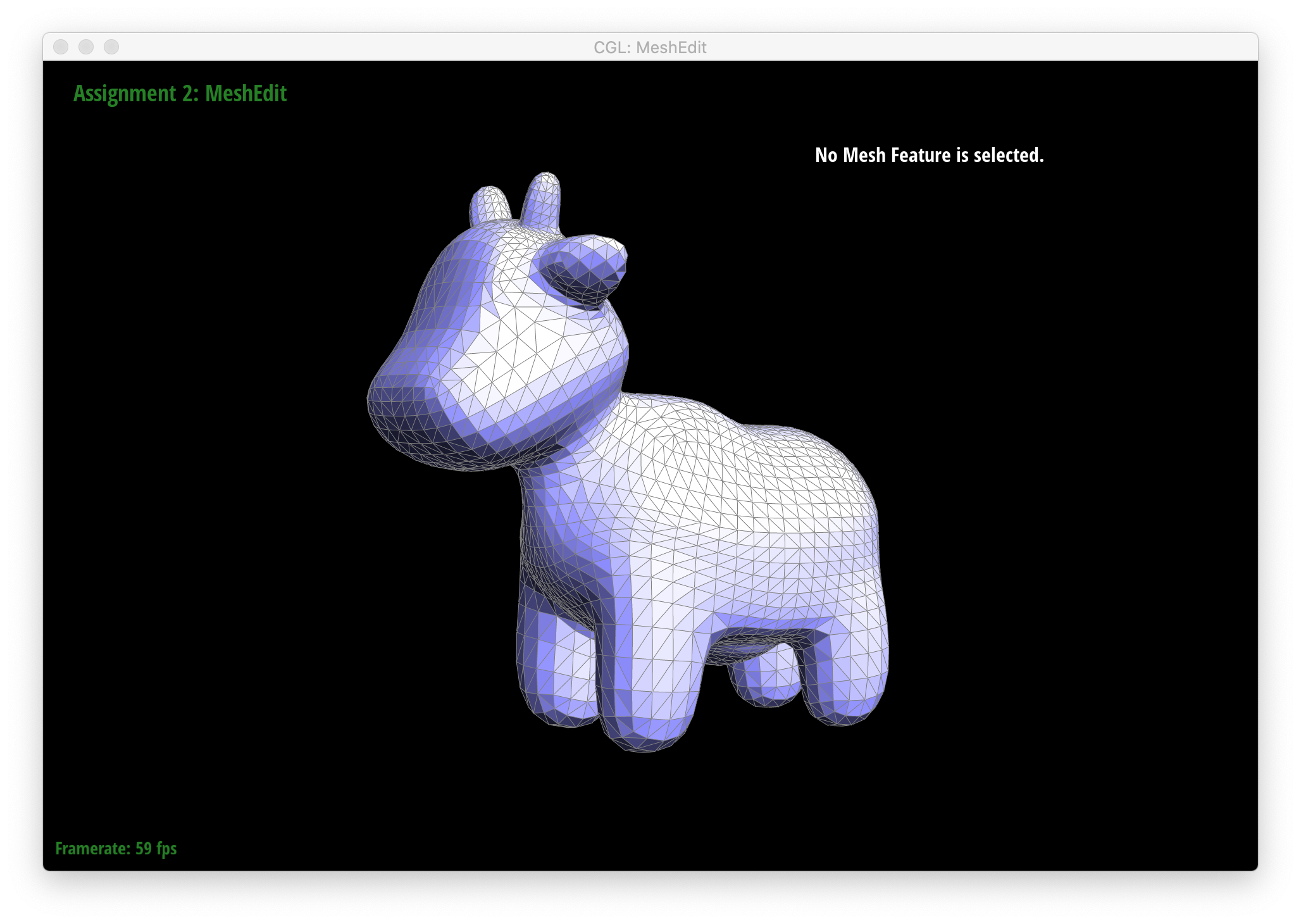
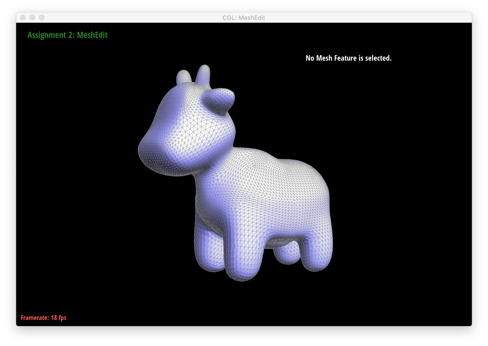
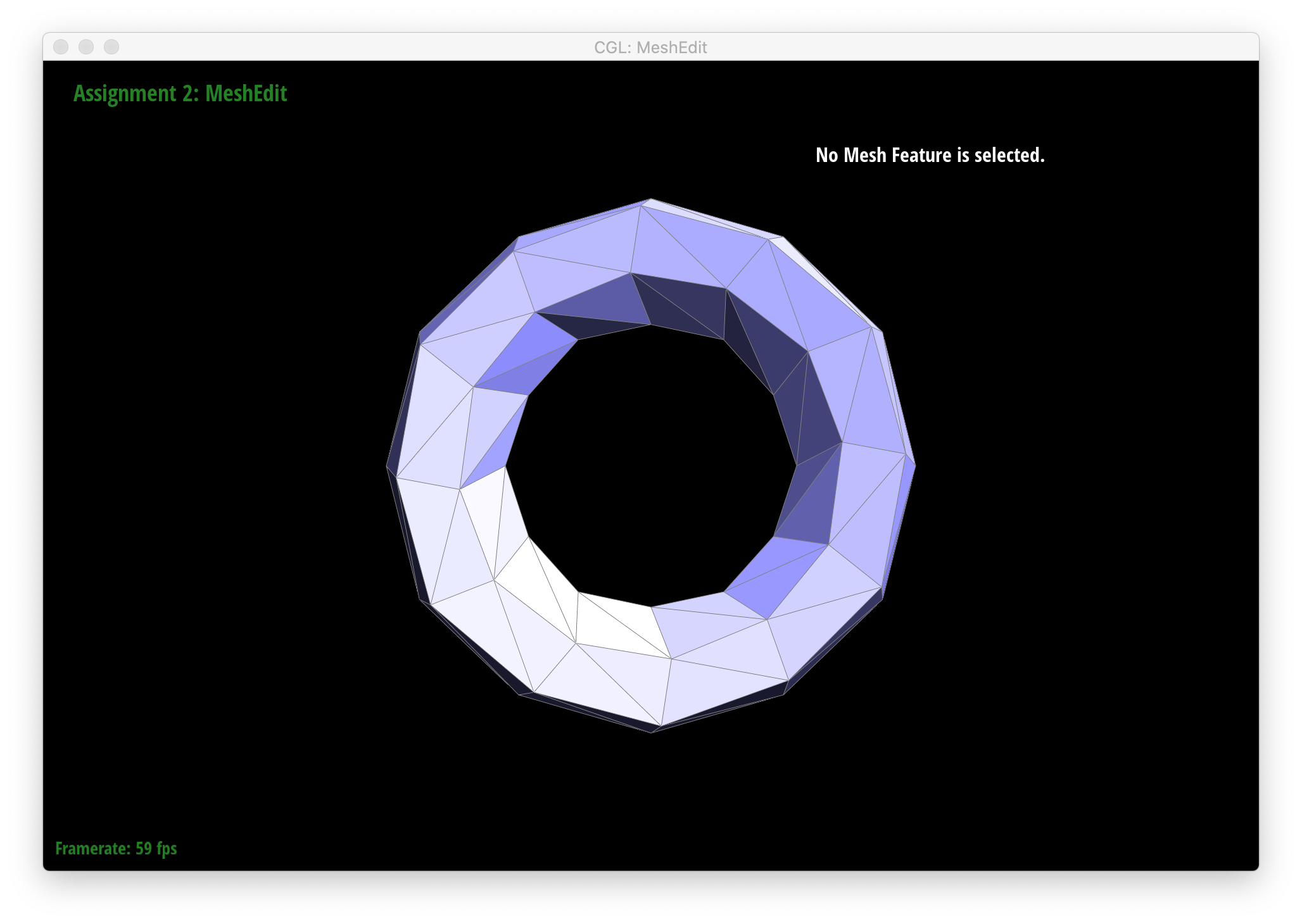
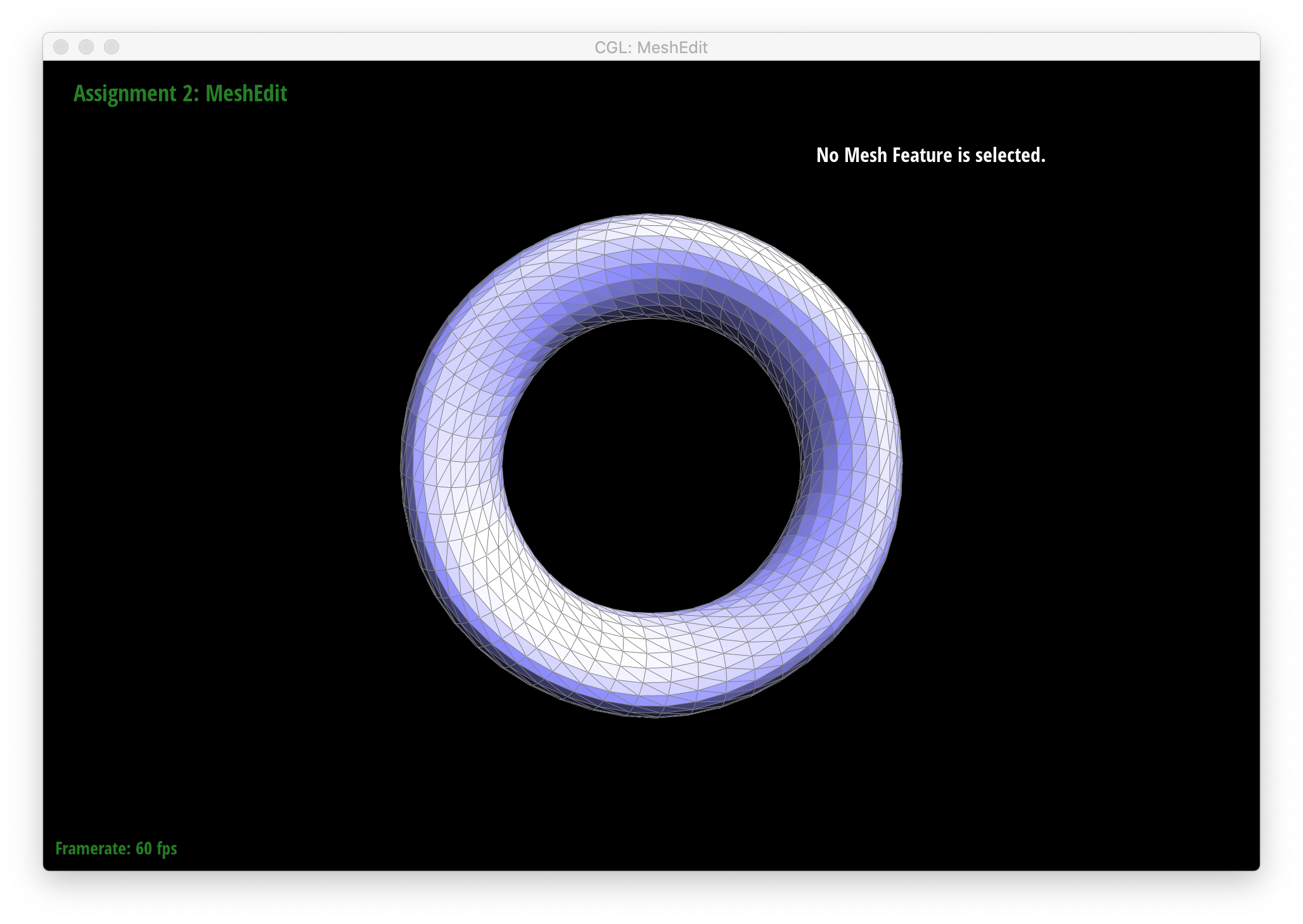
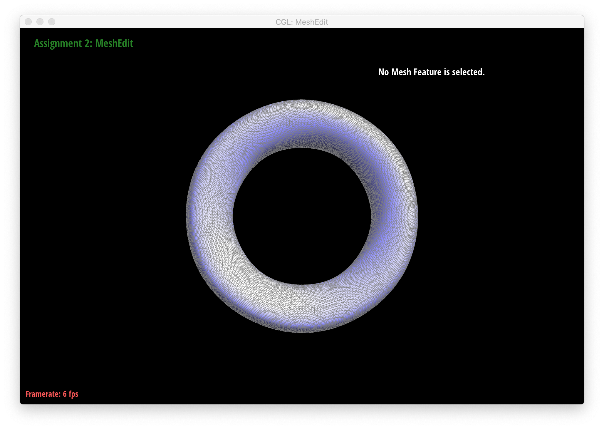
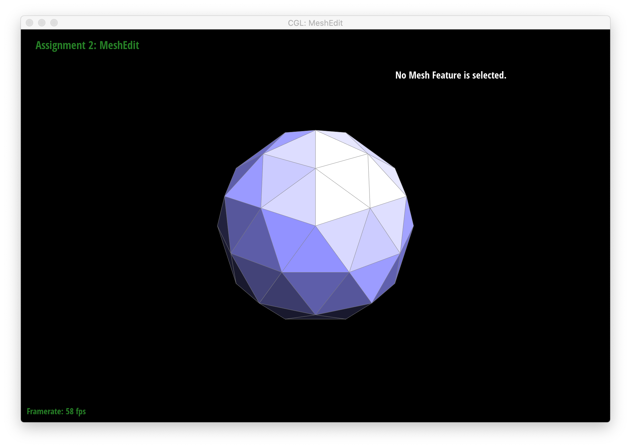
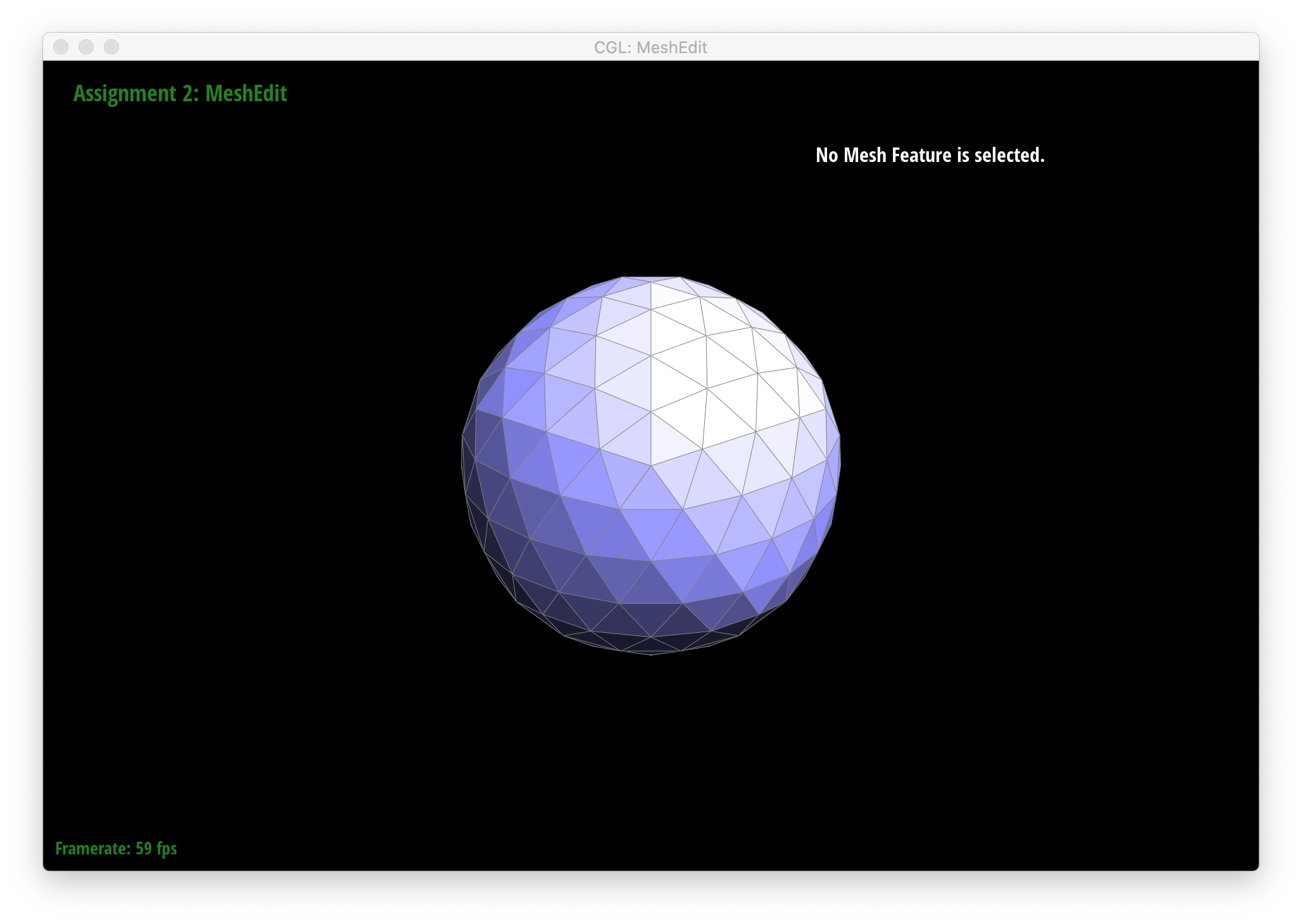
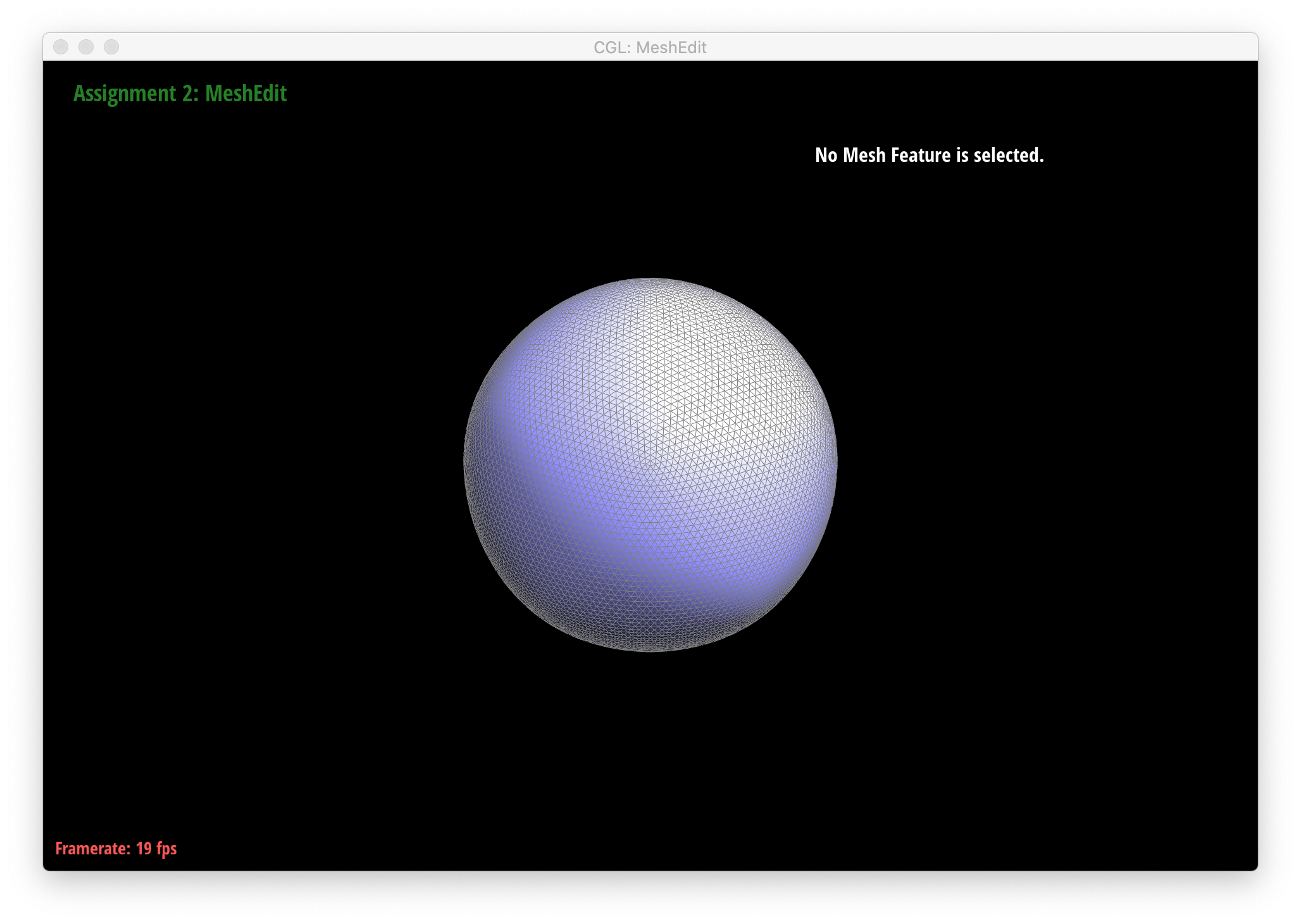
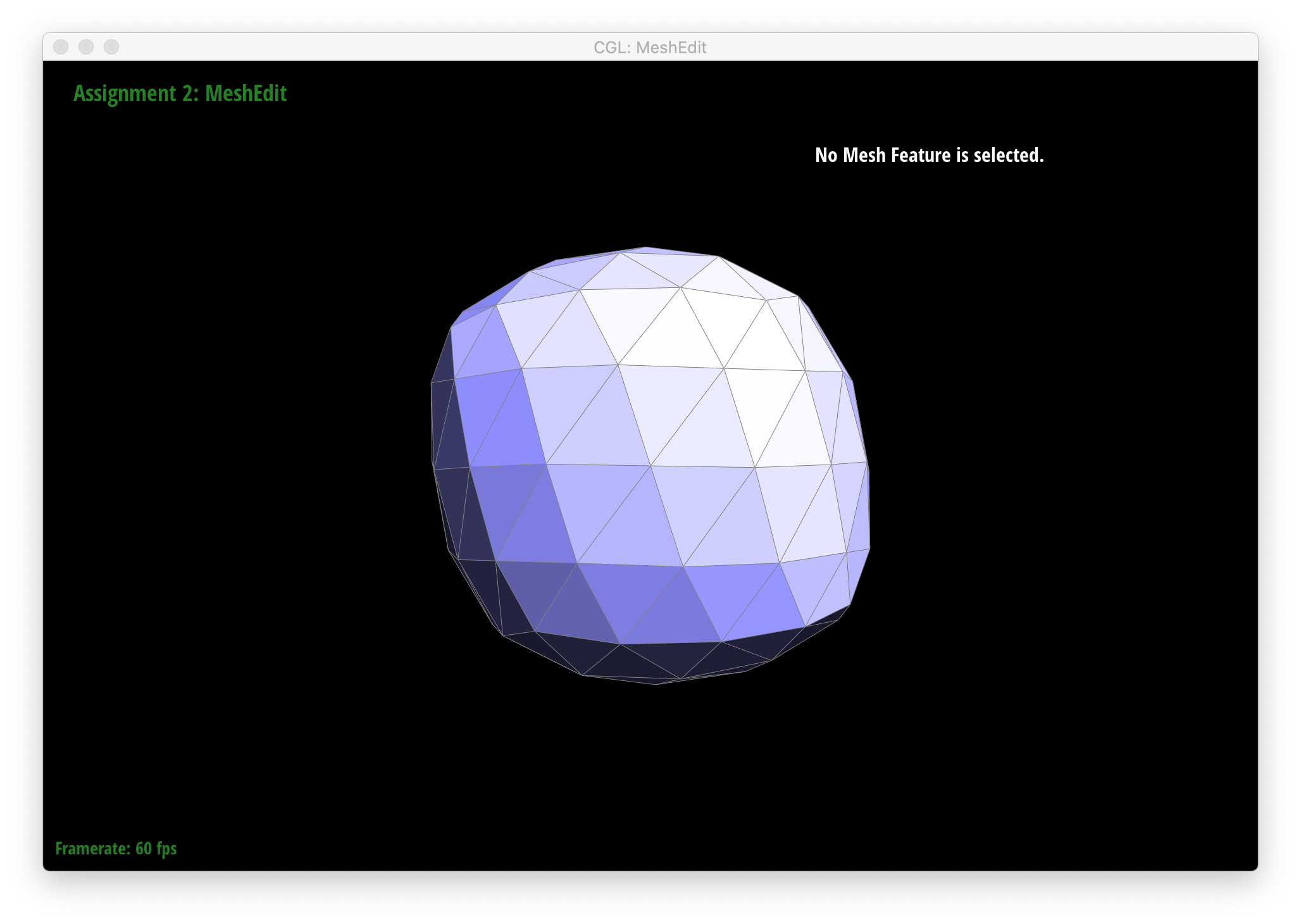
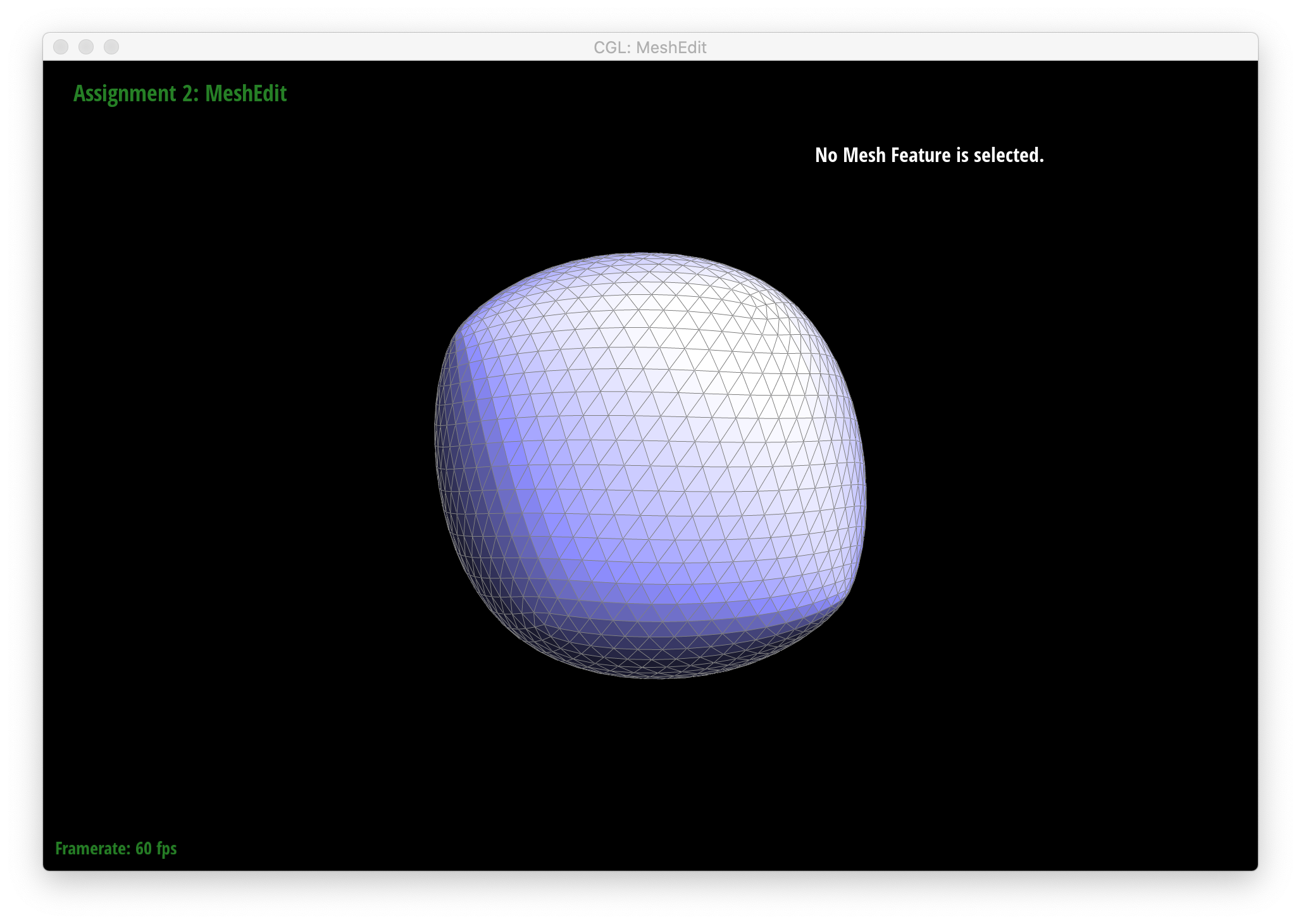
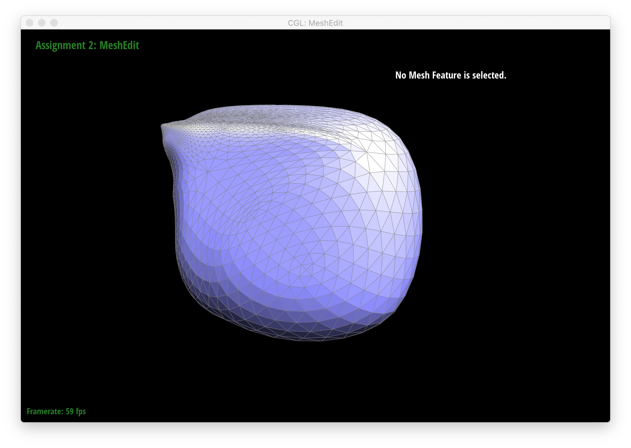
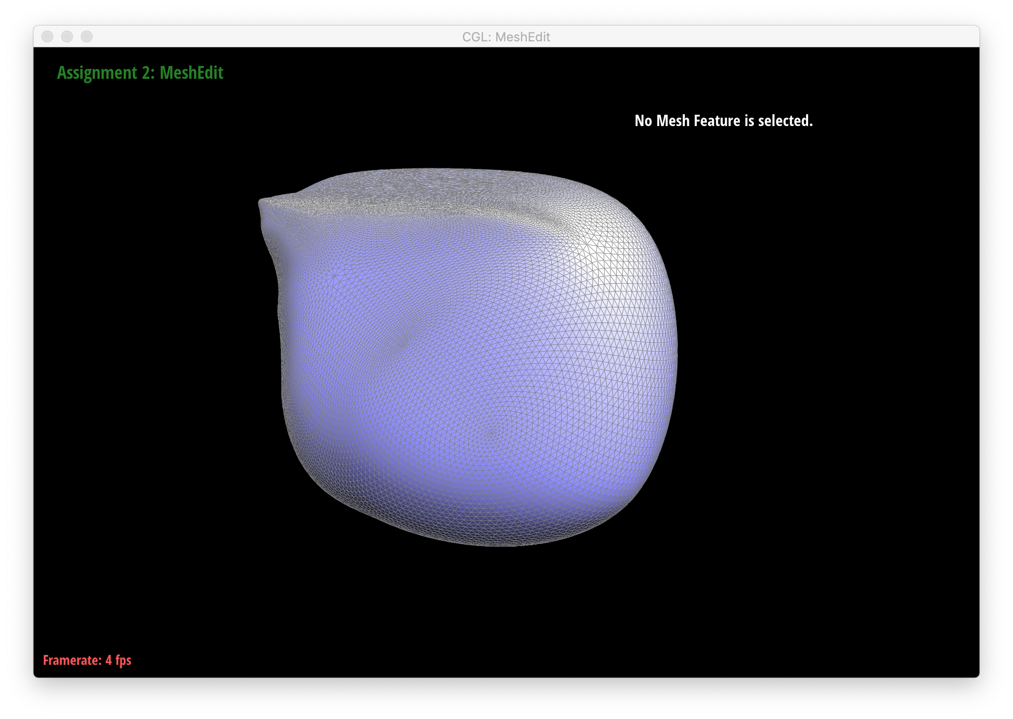
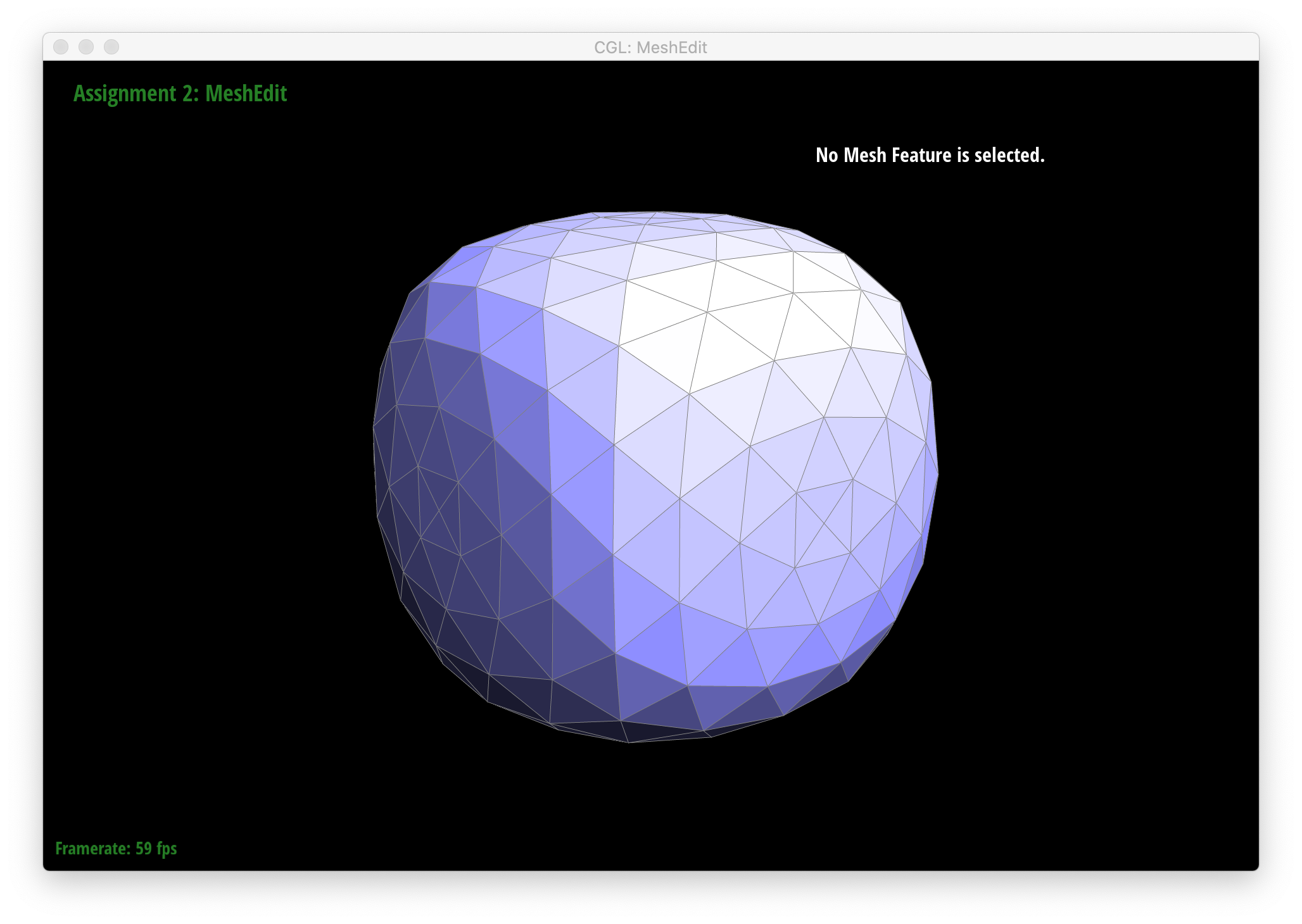
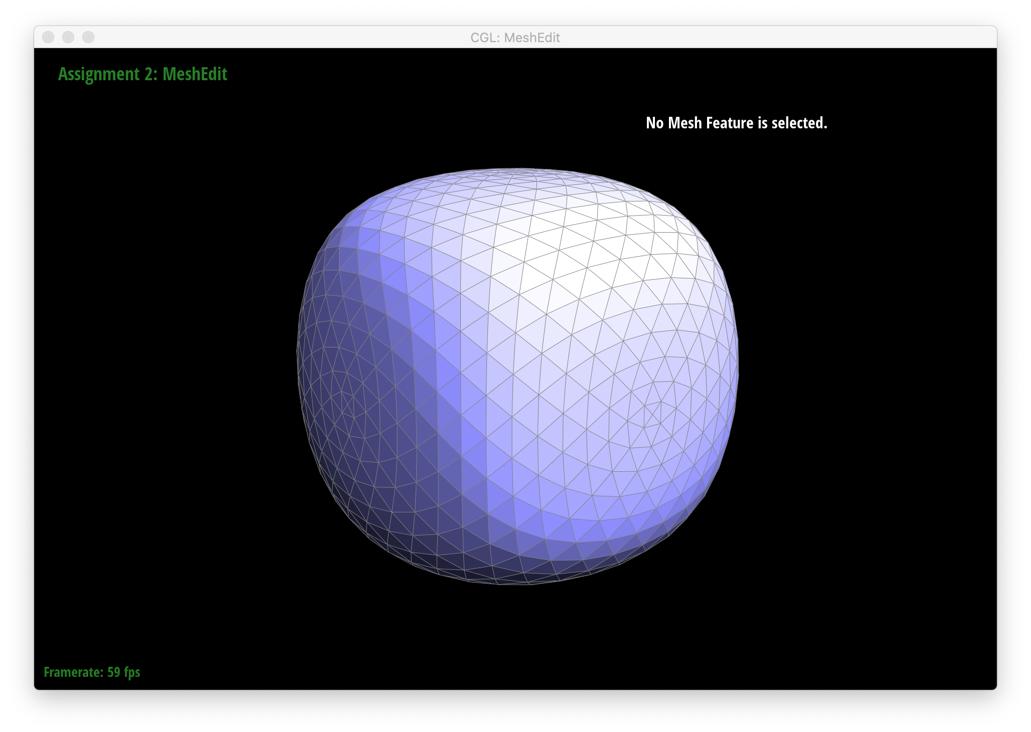
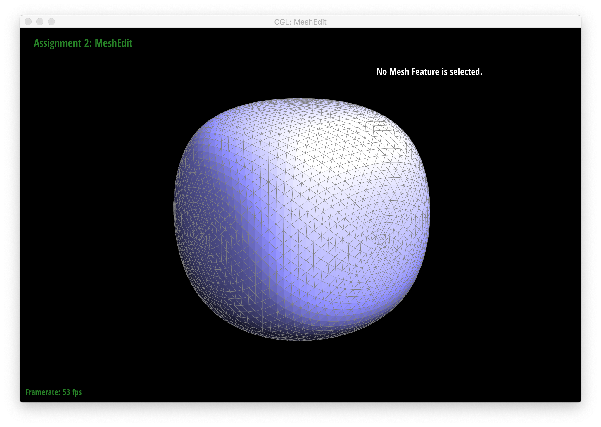
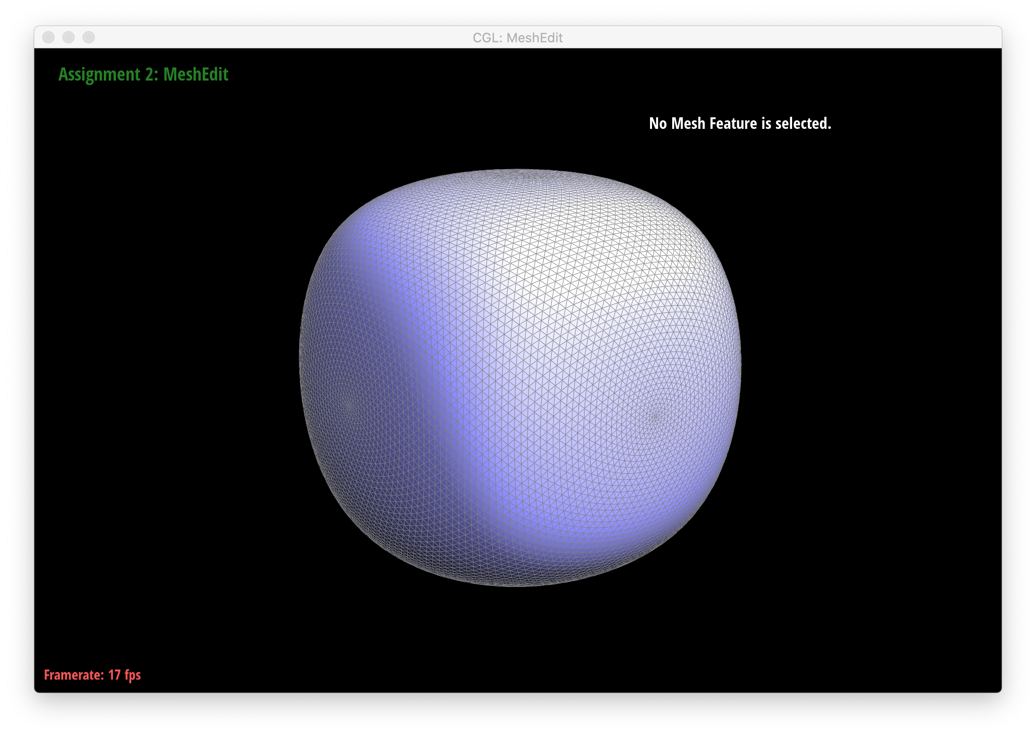
Below are screenshots of meshes after loop subdivision.

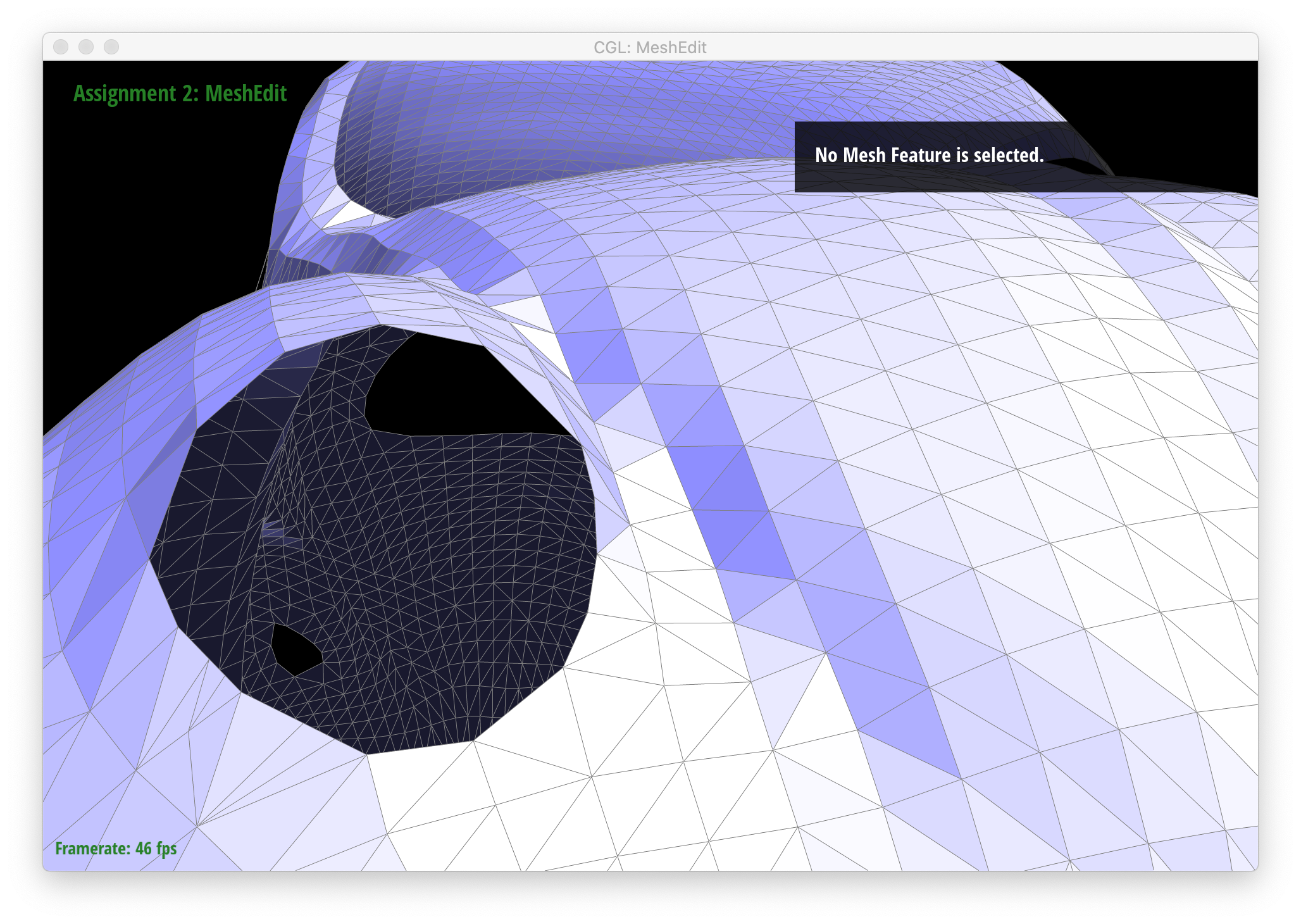
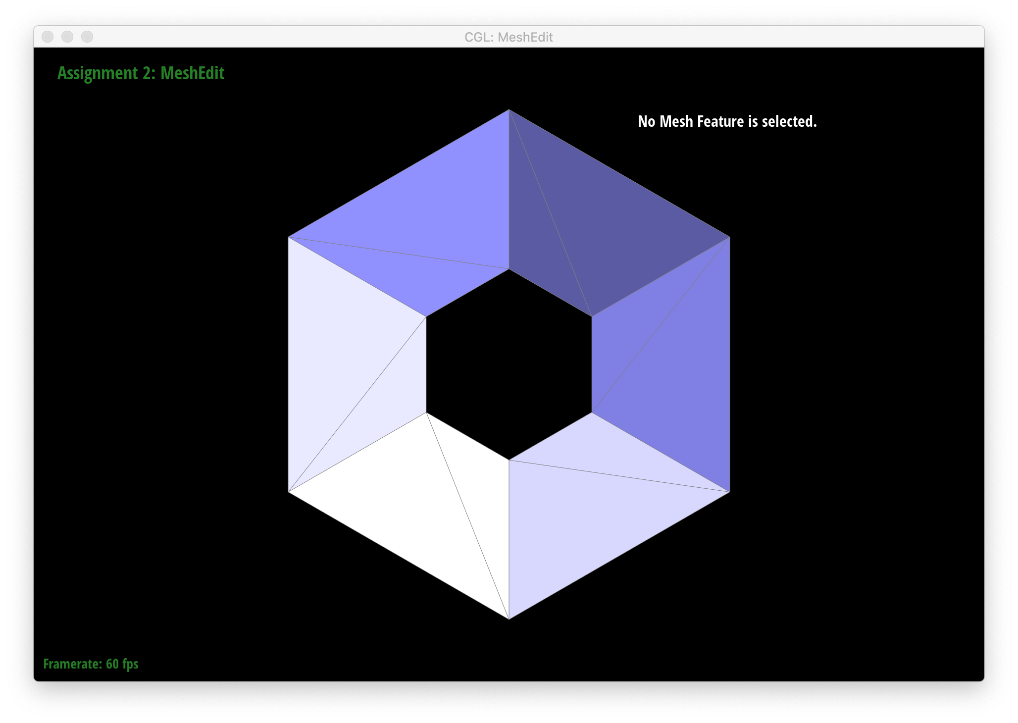
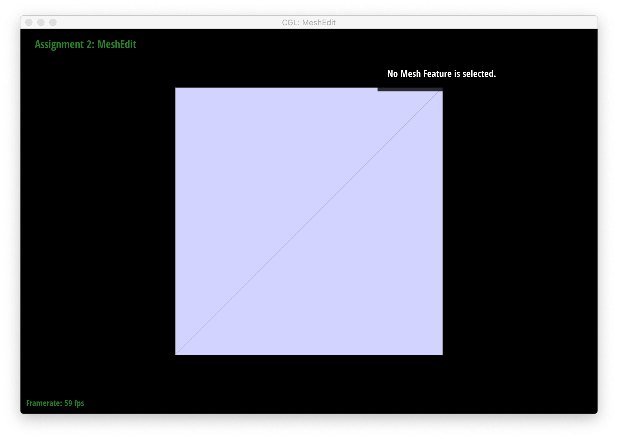
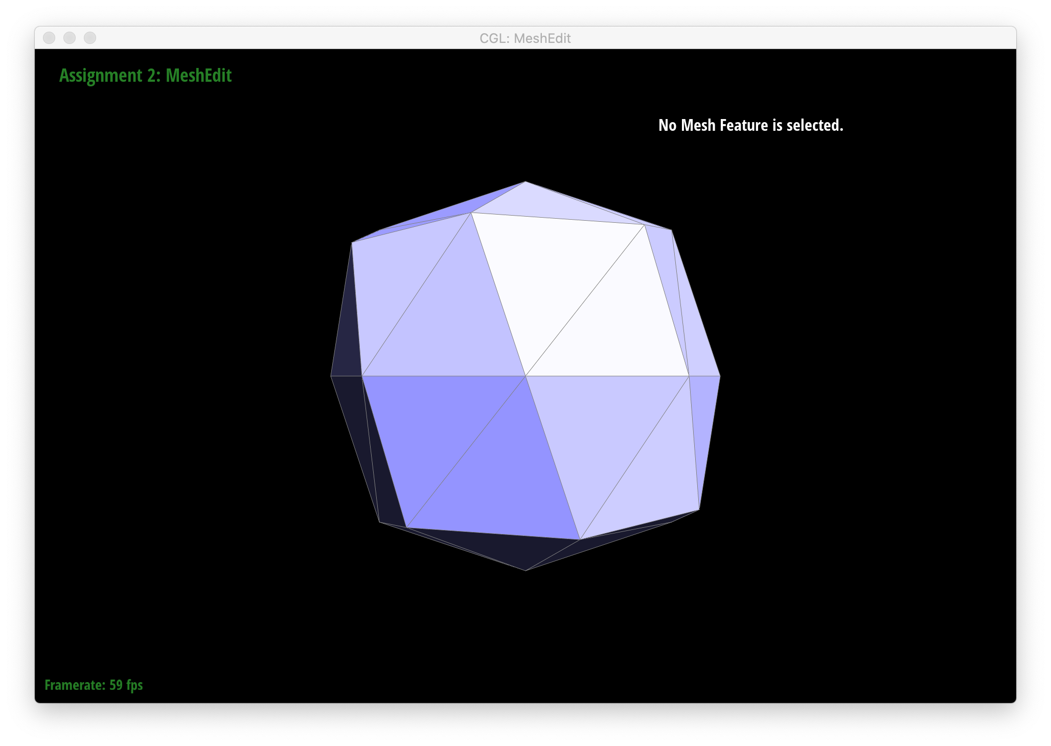
As seen in all the series of screenshots above, sharp corners and edges become dulled and smoothed with each successive round of loop subdivision. To preserve sharp features, new vertices and edges would ideally be added very close to those features during mesh upsampling to preserve the definition of those features. Placing new vertices away from sharp features would result in averaging the mesh over the sharp features (akin to an box blur filter on 2D images), reducing their sharpness. "Normal" loop subdivision without special handling for sharp edges does the latter - spacing vertices based solely on the existing mesh (which in most of the provided examples contains triangles that are largely uniform in size) and not the intended underlying features. To reduce this effect, we can increase the density of vertices around the features we want to preserve by pre-splitting some edges. An example of trying to do this around one corner of the cube .dae file is shown below:

We can see that while the rest of the cube edges and corners become smoothed and rounded as before, the one corner around which edges were pre-split to form a higher density of vertices retains much more definition.

We also see that several iterations of loop subdivision on dae/cube/input.dae result in the cube becoming slightly asymmetric. This is because successive loop subdivisions skew the mesh to follow the form and shape of the original triangles, which, in the original mesh, are not symmetric with respect to the cube's actual geometry - i.e. each square face of the cube is split in half into 2 triangles by 1 diagonal edge instead of being made up by, say, 4 triangles, which would add an axis of symmetry and thus make each loop subdivision result in a more symmetric shape. One way to remedy this is to split each edge that crosses each face of the cube such that each face is split by an "X" into 4 triangles. The resulting loop subdivision on this pre-processed mesh is shown below, and as can be seen, the cube still appears symmetric after multiple rounds of subdivision.