This assignment implements the basic elements of path tracing, which is a technique used to render scenes with realistic lighting effects, thanks to our understanding of radiometry and photometry. In path tracing, we cast rays "through" an image into a scene and use the emitted light at the point of intersection to calculate the color value to assign each pixel in the image. We can make the rendering even more realistic by accounting for subsequent ray bounces as well, using Monte Carlo path tracing, as demonstrated by later parts of this assignment. This assignment also covers core techniques to keep rendering times realistic for larger images. For example, instead of iterating over a jumbled vector of primitives when testing ray intersections, we can construct and search through a Bounding Volume Hierarchy, which drastically reduces the number of ray-primitive intersection checks for any given ray, thus leading to faster rendering time (scaling from O(N) to O(logN))! An additional algorithm, explored in Part 5, is adaptive sampling, whereby we generate fewer sample rays for "simple" pixels in the scene that converge faster than for dimmer or more complex parts of a scene. The worst part of this assignment by far was in constructing the BVH and implementing bounding box intersections. Even though the concept in some ways is much simpler than the concepts elsewhere in this assignment, properly constructing the BVH given the skeleton structure really tested my understanding of recursion, iterators, and pointers in C++. It appears that this understanding was rather rusty/non-existent to begin with, so that made debugging a rather dark journey.
Part 1: Ray Generation and Intersection
Ray Generation
Path tracing relies on the generation of sample rays from the camera through an image into the world. Ray generation (task 2 of this part) is implemented in the Camera class in the function generate_ray, which takes an input sensor sample cordinate on the plane -1 unit away on the z axis from the camera pinhole. First, the ray's bounds on t (min_t and max_t) are set to be the near and far clipping planes (nClip and fClip, respectively). Next, the ray's coordinate on the camera sensor in camera space is calculated simply using the formula (x * (sensor width) - (sensor width)/2, y * (sensor height) - (sensor height/2)), where half the sensor width/height are subtracted from each coordinate because the sensor is centered with respect to the pinhole. We can plug in sensor width = 2 * tan(0.5 * hFov) and sensor height = 2 * tan(0.5 * vFov), first converting hFov and vFov to radians, to obtain the ray's coordinate in camera space. These coordinates are then converted to world space by simply multiplying the matrix c2w with the coordinates. Finally, the new ray is assigned with an origin of the camera position, pos, and direction, in world coordinates, that were just calculated.
Ray generation is used to estimate the integral of radiance of a given pixel (task 1 of this part). More specifically, an array of random samples throughout a pixel is generated, and the camera's generate_ray function, as described above, is used to generate a ray at each one of these samples. The Pathtracer's est_radiance_global_illumination function is called on each ray, and the resulting spectrum is added to a sum. Finally, the pixel's spectrum is updated to be the average spectrum (total / the number of samples) across all samples in that pixel.
Primitive Intersection
To render a scene, we need to know if a ray intersects a primitive in that scene. Primitive intersection is implemented in each primitive class (here, Triangle and Sphere). Each class has a has_intersection function that tests whether a ray, passed in as input, has a valid intersection with that primitive. It may do this by setting the ray vector, r(t) = o + t * d, where o is the ray's origin and d is the ray's direction (stored in the Ray structure), as a point in the implicit equation that describes the primitive, and then solving for the t that allows that equation to still hold true. For example, a sphere (task 4 of this part) may be described as all points p that satisfy the equation (p - c)^2 - R^2 = 0, where c is the sphere's origin and R is the sphere's radius. The ray's intersection with the sphere is then found by setting p = r(t) = o + t * d and solving the resulting quadratic equation for t. For the case of the sphere in particular, this will yield 2 values of t. If the smaller t is between the ray's min_t and max_t, then a valid intersection at that smaller t has been found. Otherwise, if the larger t is between the ray's min_t and max_t, then a valid intersection at that larger t has been found (since we are concerned with the closest intersection, we don't worry about the larger t for this part if the smaller t already yields a valid intersection). In the function intersect, if a valid intersection is found, the ray's max_t variable is updated to be the found t. Additionally, the Intersection's t, primitive, bsdf, and n variables are updated to be the found t, this (the current primitive), the current primitive's bsdf as found by get_bsdf(), and the normalized normal vector at that point of intersection (i.e. the ray's value at the found t, r(t) minus the ray's origin), respectively.
Triangle Intersection
For triangle insersection (task 3 of this part), I use the Möller Trumbore algorithm to determine in the Triangle's has_intersection function whether the ray passed in as input intersects the given triangle. The Möller Trumbore algorithm is more efficient than testing if a given point lies on the same side of all 3 of a triangle's edge, and this becomes important later on in the assignment when tasks start becoming more complex. The algorithm starts by setting the ray equation, r(t) = O + t * D, equal to the equation for a point P within a triangle: P = (1 - b1 - b2) * P0 + b1 * P1 + b2 * P2. We can convert this equality to the form Mx = b, where M = [-D, P1 - P0, and P2 - P0], x = [t, b1, b2], and b = O - P0. The equations for the Möller Trumbore algorithm are derived by using Cramer's rule to solve for x = 1/|M| * [|M1|, |M2|, |M3|], where Mi is M with its i-th column replaced by b. This yields the final equations (presented in lecture) that takes the points of the triangle, P0, P1, and P2, and the ray's origin O and direction D to find t, b1, and b2. A valid intersection is found if t is valid (i.e. it is between the ray's min_t and max_t) and if b1 and b2 are valid (i.e. b1 >= 0, b2 >= 0, and (1 - b1 - b2) >= 0, since these are the barycentric coordinates of the found point). In Triangle's intersect function, if has_intersection returns true, then the ray's max_t is updated to be t, and the Intersection passed in as an input is updated just as described in the sphere case above, except its normal is calculated using the Barycentric coordinates of the point of intersection with respect to the triangle's vertex positions. Conveniently, b1 and b2 from the Möller Trumbore algorithm are already 2 out of the 3 Barycentric coordinates, corresponding to the v2 and v3 vertices of the triangle, respectively. The Barycentric coordinate corresponding to the triangle's vertex v1 is then simply 1 - b1 - b2, and the normal vector at the point of intersection is thus (1 - b1 - b2) * n1 + b1 * n2 + b2 * n3, where n1, n2, and n3 are the normal vectors at the triangle vertices v1, v2, and v3, respectively.
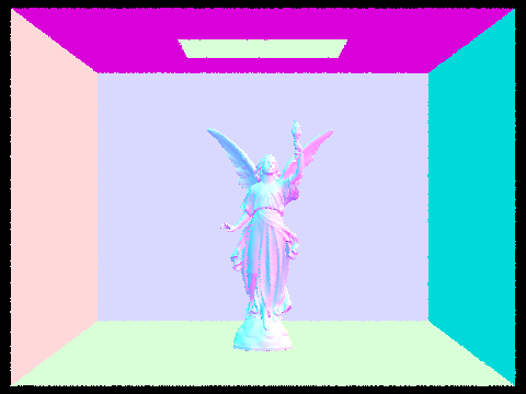
Below are some images with normal shading for a few .dae files (1 sample/pixel).
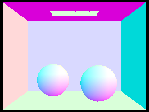
/dae/sky/CBspheres.dae with normal shading
|
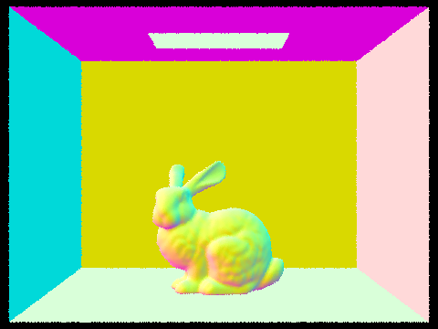
/dae/sky/CBbunny.dae with normal shading
|
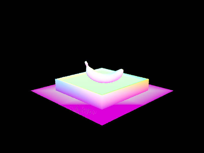
/dae/keenan/banana.dae with normal shading
|
Part 2: Bounding Volume Hierarchy
Bounding Volume Hierarchies (BVH) are data structures that drastically improve the efficiency of testing ray-primitive intersections and thus improve rendering times. In a BVH, a root node contains all primitives in the scene. It also points to a left and right child node, with one node containing the primitives on one side of a spatial plane and the other node containing the primitives that lie on the other side of that plane (more on this below). The children nodes similarly have their own left and right child nodes that each split the primitives in that node into two, until the nodes at the bottom of the tree contain at most max_leaf_size nodes, as specified by the program.
My BVH is constructed recursively in construct_bvh. First, a bounding box for the node is constructed by adding all the primitives between the given start and end pointers. If the number of primitives is at most max_leaf_size, the node is a leaf node - i.e. its start and end iterators are assigned to be the input start and end, and it's l and r node pointers are left null. Otherwise, the node is split. The x, y, and z spans of the node's bounding box are obtained from the bounding box's extent variable and compared. The primitives in the node are sorted in ascending order along the axis of maximum extent. This is done with the sort function, using custom helper functions compareX, compareY, or compareZ, depending on whether primitives are being sorted by x, y, or z. I [somewhat arbitrarily] chose the split point to be the centroid of the node's bounding box. This is a fairly simple-to-implement heuristic that is especially effective for somewhat uneven/lopsided spatial distributions, as it avoids encapsulating empty space within a single node that would otherwise increase the expected cost of ray-primitive intersection later on. The vector of primitives is traversed until the primitive has a centroid coordinate (in the bounding box's longest axis) that is greater than the split point. This point is assigned a new iterator, middle. If middle is not between (start, end), this indicates that all primitives lie on one side, so middle is arbitrarily set to the midpoint between start and end to split the node into even halves. To construct the left node, construct_bvh is recursively called with start and middle as the start and end iterators, and the right node is constructed similarly by calling construct_bvh with middle and end as the start and end iterators.
With this structure, we don't have to go through every primitive and test if the ray intersects it. Instead, we first test if a ray intersects the root node's bounding box, which is implemented in bbox.cpp's intersect function. That function finds the minimum and maximum times that an input ray passes through that bounding box, if it does at all, and returns them if they are in the valid range (provided as input to the function). It also returns true if the ray is contained entirely within the bounding box, which becomes important for later parts of this assignment. If the ray intersects the root node's bounding box, we check if the ray intersects that node's left and right children's bounding boxes. If it only intersects one, we know that we only have to search in that child's bounding box, and we recursively do so until we enter a leaf node, at which point we perform a ray intersection test on every primitive in that leaf (just max_leaf_size tests!) and update the ray's max_t and nearest intersection's variables. If at any level of recursion, the ray intersects both children's bounding boxes (call them A and B), we first check the child A node with the bounding box for which the nearest intersection is closer and recursively check bounding boxes underil we enter a leaf node to find the nearest intersection. If that nearest intersection time point occurs before the ray intersects the other B node's bounding box, we don't even have to enter that other B node at all. Otherwise, we similarly search the B node (and recursively its children down to the appropriate leaf node), and if a nearer primitive intersection is found there, the ray's max_t and input intersection's variables are updated.
Images with normal shading for cow.dae, maxplanck.dae, beast.dae, and CBlucy.dae are shown below. The last 3 images are large enough that they can only realistically be rendered with BVH acceleration.

/dae/meshedit/cow.dae with normal shading and BVH acceleration
|

/dae/meshedit/maxplanck.dae with normal shading and BVH acceleration
|
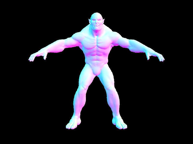
/dae/meshedit/beast.dae with normal shading and BVH acceleration
|
/dae/sky/CBlucy.dae with normal shading and BVH acceleration
|
Rendering time comparisons for a few scenes with moderately complex geometries with and without BVH acceleration are below. This was done on my personal computer (2019 MacBook Pro) with 8 threads and other parameters left as the default. The benefits of BVH are especially great on structures of very large numbers of primitives. Ray tracing without acceleration scales with N as O(N), but with BVH, this is reduced to O(logN). With BVH, a very few number of leaf nodes (usually just 1) must be entered and traversed for ray-primitive intersection, so the average number of intersections per ray will be just above the max leaf size (this was reported during the below tests as an average of ~1.5 intersections/ray, but this number is not entirely accurate because the incrementing of the variable total_isects is not thread-safe. Realistically, BVH acceleration reduces the number of ray-primitive intersection tests per ray to just above max_leaf_size.
| COLLADA file | Rendering time, baseline | Rendering time with BVH acceleration |
| cow.dae | 30.4963s | 0.0277s |
| maxplanck.dae | 299.6330s | 0.0365s |
| CBbunny.dae | 54.3083s | 0.0418s |
For some reason, when within a leaf node, I at first was doing ray-primitive intersections with every single primitive in primitives when I meant to be only testing intersections with primitives within that leaf node. I spent 3 days (ouch) trying to figure out why my code only achieved modest improvements in rendering speeds, and in the process, I ended up adding a few extra smaller optimizations that made my code even zippier than I expected when I finally fixed my bug. For instance, when both a left and right bounding box have intersections, the closest one is entered first, and only if there's a possibility that the "farther" bounding box has a closer primitive intersection is it entered (i.e. if the farther bounding box's minimum intersection is closer than the found intersection in the closer bounding box). Also, as a smaller optimization, in the bounding box intersection tests, I make use of the Ray structure's inv_d variable to multiply by pre-calculated slope inverses instead of doing the more expensive division operation for every time calculation.
Part 3: Direct Illumination
In task 1, the DiffuseBSDF::f and DiffuseBSDF::sample_f functions are implemented. Because the BSDF of diffuse materials does not depend on incoming/outgoing direction, f simply returns a constant albedo (reflectance) / pi, to normalize over the quarter sphere from which an incoming ray may reflect. In sample_f, the pointer wi is assigned to a sample direction via the sampler's get_sample function with the pdf as an input. f with the input wo and sampled wi is then returned.
For the first implementation of the direct lighting function, we estimate the direct lighting on a point by sampling uniformly in a hemisphere. This is implemented in estimate_direct_lighting_hemisphere, which is in turn called by one_bounce_radiance. For uniform hemisphere sampling, we set the number of samples to be equal to that used when importance sampling the light (detailed below) for comparison. For each sample, a sample direction in object space, wi, is generated with the hemisphereSampler's get_sample function. We then create a sample (shadow) ray. This ray's origin is given by the hit point, hit_p in world space with an additional epsilon in the direction of travel, which is given by EPS_D times the sample direction in world space (o2w is appled to the sample direction). This offset is to avoid precision errors and intersections with hit_p. Next, a new Intersection is created, and the BVH's intersect function is used to check if the sample ray makes any intersections in the scene. If it does, the spectrum L_i at that point is found by that intersection's bsdf->get_emission(). As the reflection equation suggests, L_i's contribution to the total emission L_out is then multiplied by isect's bsdf's f given wi and w_out and cosine(theta), which is just the z-component of wi in object space, since the object normal is (0,0,1). For all the sample rays generated, these terms are summed, and at the end, the final spectrum is this sum normalized by dividing by the number of samples and the pdf, the latter of which is just 1/(2pi) in the case of uniform sampling over a hemisphere.
For the second implementation of the direct lighting function, we use importance sampling of all the lights to reduce noise and also be able to render images with point lights (which have a near-zero chance of being sampled with uniform hemisphere sampling). This is implemented in estimate_direct_lighting_importance. For each light in the scene, we sample a light num_samples times. If the light is a point source, num_samples = 1, and otherwise, num_samples = ns_area_light. For each sample, the light's sample_L function is used to determine (1) world_dir, the direction (a unit vector in world space coordinates) from the point of intersection, hit_p, to a sample on the light, (2) distToLight, the distance to the light in the direction of world_dir, (3) pdf, the pdf evaluated in the world_dir direction, and (4)L_i (L_o in the lecture slides), the outgoing radiance from the light point. I chose these variable names to match those in estimate_direct_lighting_hemisphere to help keep concepts straight in my mind. The sample_L function already takes into account the "change in basis of integration" terms that arise from integrating over the area of the light (i.e. dw = dA'cos(theta')/(p'-p)^2)), so we're ready to use world_dir as it was used in hemisphere sampling. The wi vector in object space is generated by applying the w2o matrix to world_dir, and cos_theta is again simply wi's z component. If cos_theta < 0, the light is behind the surface at the hit point, so we continue to the next sample. Otherwise, a shadow ray is generated with hit_p plus an epsilon (in the direction of world_dir) as the origin and world_dir as the direction. The ray's max_t is set to be distToLight, because we aren't interested in intersections that happen beyond the light. If the ray doesn't intersect anything else in the scene, it has a direct line of sight to the sampled point of the light, so the contributed emission ( = L_i * (the isect's bsdf's f given wi and w_out) * cos(theta) / pdf) is added to a running sum emission, L_out. Finally, the emission is normalized by dividing by the number of samples taken.
Below are some images rendered with both uniform hemisphere sampling and lighting sampling. All were generated with 64 camera rays/pixel and 32 samples/area light. More comments on dragon.dae and other point light-only scenes are at the end of the section.

CBbunny.dae, uniform hemisphere sampling |
CBbunny.dae, importance lighting sampling |
 CBspheres_lambertian.dae, uniform hemisphere sampling |
 CBspheres_lambertian.dae, importance lighting sampling |
 dragon.dae, uniform hemisphere sampling |
 dragon.dae, importance lighting sampling |
Below are images of CBbunny.dae rendered with 1, 4, 16, and 64 light rays and 1 sample per pixel using light sampling. The noise levels in soft shadows clearly improves as the number of light rays increases. As we take more samples, we better approximate the "true" shape of the shadow. Variance is inversely proportional to the number of samples.

CBbunny.dae, 1 light ray/area light
|

CBbunny.dae, 4 light rays/area light
|

CBbunny.dae, 16 light ray/area light
|

CBbunny.dae, 64 light rays/area light
|
Uniform hemisphere sampling and lighting sampling both can render many scenes with direct lighting, but as can be seen above, uniform hemisphere sampling is noisier for the same parameters than lighting sampling. This is because the probability of actually hitting a light source from random rays cast across a uniform hemisphere is in general quite low, which results in more dark spots that appear as noise in the final image. Additionally, for scenes with only point light sources, the probability of sampled rays hitting the light source is nearly zero, so these scenes appear dark. Such is the case for scenes like dragon.dae, as seen above.
Part 4: Global Illumination
The images generated in Part 3 are certainly fairly realistic, but they are missing elements of "real" scenes that arise from a light ray bouncing through a scene instead of just once. The at_least_one_bounce_radiance function allows us to render global (direct + indirect) illumination effects with Monte Carlo estimation. It is a recursive function that terminates if the input ray depth is < 1. Otherwise, the emitted light is first set to the one_bounce_radiance for the input ray r and intersection isect - this is the effect from direct illumination described in Part 3. coin_flip is used to implement termination by Russian Roulette and takes as input the probability that the function should return 1. I chose to use 0.7 as this probability (i.e. the cpdf). If the coin_flip returns true, then we haven't terminated yet, so the algorithm continues. The bsdf at isect is obtained with the bsdf's sample_f function, which takes in w_out and updates the wi and pdf at that hit point. As in the one_bounce_radiance function described previously, a new ray is generated from the hit point (+ the same epsilon) with a direction obtained by applying the o2w matrix to wi. This ray's depth is one less than that of the ray that was input into the call toat_least_one_bounce_radiance. If this new ray intersects the scene (checked with the BVH's intersect function), its contribution to the total emitted light is added. Similar to before, this is equal to L_i * f * cos_theta / pdf / cpdf. Notable differences are that (1) there is an additional cpdf term that we normalize by to account for Russian Roulette termination, and (2) L_i is not a calculated/sampled emission but is rather a call to at_least_one_bounce_radiance with the new ray and new intersection points as input. In the case when the initial ray depth was 1, the recursion will terminate on the next round before L_out is updated, so L_out will simply be the output of one_bounce_radiance, as expected. Otherwise, this recursion simulates a light ray bouncing through a scene from one object to another.
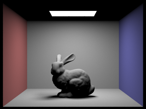
Below are some images rendered with global (direct and indirect) illumination, using 1024 samples per pixel, 4 light rays/area light, and max_ray_depth = 5.

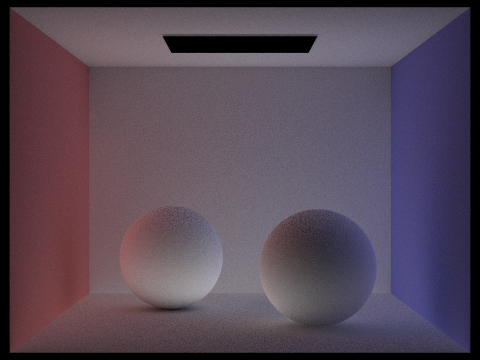
CBspheres_lambertian.dae
|

CBbunny.dae |
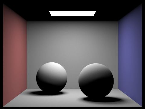
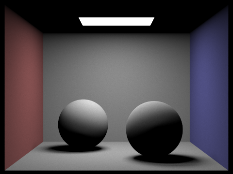
Below is a comparison of CBspheres_lambertian.dae rendered with only direct illumination and only indirect illumination (the latter is achieved by subtracting the effect of one_bounce_radiance from L_out). Both images use 1024 samples per pixel, 4 light rays/area light, and max_ray_depth = 5. We see that the effects of indirect illumination allow us to achieve certain global illumination effects such as color bleeding (reflection onto the spheres and walls of the colored walls) and more realistic shadows (the shadows under the spheres aren't just huge black blobs).
CBspheres_lambertian.dae, direct illumination only
|
CBspheres_lambertian.dae, indirect illumination only
|
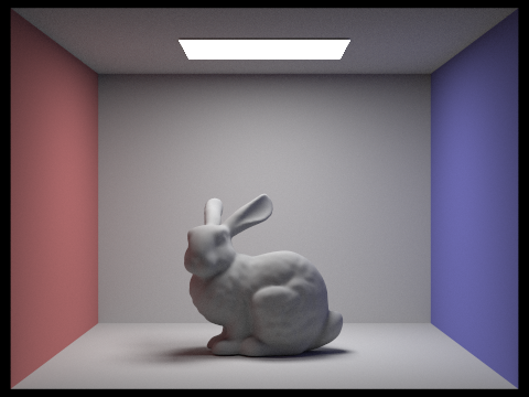
Below are rendered views of CBbunny.dae with 1024 samples per pixel, 4 light rays/area light, and max_ray_depth set to 0, 1, 2, 3, and 100. For max_ray_depth = 0, we simply get the zero-bounce radiance, or only the area light. For subsequent max_ray_depths, the greater the maximum ray depth is, the more average bounces we integrate over, and the more realistic (and brighter) a scene becomes, though this has diminishing returns because the amount of light reflected with each bounce decreases. Increasing the max_ray_depth does come a slight (thankfully greatly mitigated by Russian Roulette termination) rendering time. For example, for max_ray_depth = 1, the scene takes 200 s with 8 threads on my Macbook Pro. For max_ray_depth = 100, the scene takes 453 s.
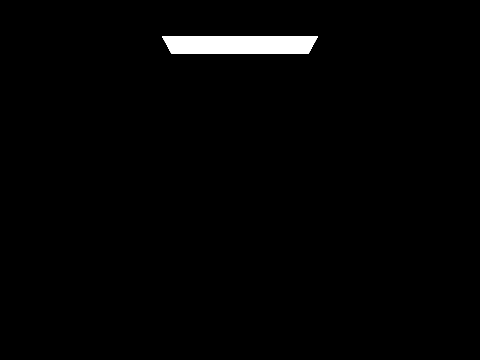
max_ray_depth = 0
|

max_ray_depth = 1
|
max_ray_depth = 2
|
max_ray_depth = 3
|

max_ray_depth = 100
|
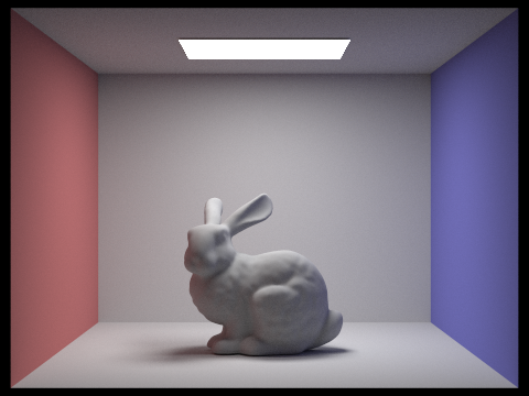
Below are rendered views of CBbunny.dae with various samples-per-pixel values. All images use 4 light rays and max_ray_depth = 5. The number of samples per pixel greatly influences rendering time and quality. For 1 sample/pixel, the image is very noisy and speckled, as intuitively, there is a lot of error when a single sample ray shot into the scene (that is subsequently terminated with some probability according to the cpdf) is used to describe the color assigned to that pixel. Increasing the number of samples per pixel greatly improves this quality, faster in well-lit areas but also for low-lit areas/features. By the time we're taking 1024 samples/pixel, elements in the image appear smooth with almost no noticeable noise in any particular area. Rendering time scales linearly with the number of samples, however, so it can quickly become expensive if one needs high-quality images. The first image with 1 sample/pixel took 0.3513s on my machine to render, while the image with 1024 samples/pixel took 422 s.
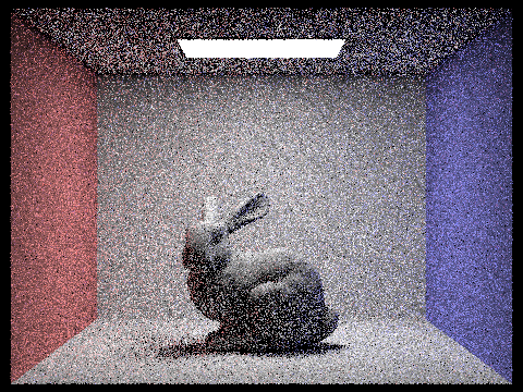
1 sample/pixel
|
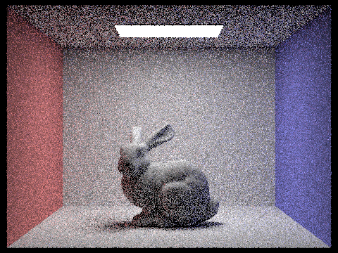
2 samples/pixel
|
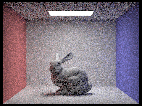
4 samples/pixel
|

8 samples/pixel
|

16 samples/pixel
|
1024 samples/pixel
|
Part 5: Adaptive Sampling
As seen above, Monte Carlo path tracing can be effectively used to generate realistic images, but images tend to be noisy unless a large number of samples/pixel are used. This can be very slow for large images. Adaptive sampling is a technique to more "smartly" sample pixels such that we don't waste time using a high number of samples per pixel for "easy" areas of the image that converge with far fewer samples, but we can still use a high number of samples to improve quality for pixels with inherently noisier signals.
To implement adaptive sampling, I modify the sample ray-generation loop of the raytrace_pixel function of the pathtracer. For every sample, we calculate the spectrum of our sample ray as usual. We find the illuminance associated with that spectrum using the spectrum's illum function and add that to running sums s1 and s2, which are variables that we use to calculate standard deviation later. For s1, we simply add the illuminance, and for s2, we add the illuminance squared. When the number of samples taken, n, is a multiple of the input samplesPerBatch parameter (found by checking if the number of samples % samplesPerBatch == 0), we check for convergence. We do this by calculating the mean of the n samples, which is s1/n, and the standard deviation sd, which is 1/(n-1) * (s2 - s1^2 / n). We then calculate the parameter I, which decreases with the samples' variance (= squared standard deviation) and/or the number of samples, and use a z-test to check if the average illuminance in the pixel so far is between mean - I and mean + I with 95% confidence. We do this check by checking if I = 1.96 (which comes from deciding to check with 95% confidence) * sd / sqrt(n) <= maxTolerance * mean. If so, this means that we are confident that our variance is "small enough," and we can stop sampling here and just update the pixel to be the average of the samples taken thus far. The sampleCountBuffer is also updated to reflect the actual number of samples for that pixel so that the sampling rate image can be rendered.
Below is CBbunny.dae rendered with up to 2048 samples/pixel, 1 sample/light, and a max ray depth of 5. Also included is the sampling rate image that shows clear visible differences in sampling rate over various regions and pixels. Areas such as the shadows and darker features of the bunny are "hard" areas to render and require a high number of samples per pixel to render, which is why they show up as red in the sampling rate image. Conversely, large areas of the wall and areas that are more lit are easier, less complex areas to render and will converge with a fewer number of samples, which translates to being green in the image. The area light itself and area outside the Cornell box converge virtually instantly, which is why they appear blue (lowest number of samples/pixel) in the sampling rate image.

CBbunny.dae, rendered with adaptive sampling
|

CBbunny.dae, adaptive sampling rate map
|