This assignment continues exploring elements of a pathtracer that can be used to render photorealistic scenes. For this assignment, I wanted to gain some experience with both advanced material modeling and implementing more realistic camera effects, so I chose to implement microfacet material modeling (part 2) and the depth of field effect (part 4). After being introduced to path tracing and material modeling in Assignment 3-1, modeling microfacet materials wasn't such an alien concept, and it was satisfying to see how modulating terms based on real-world data could influence the appearance of rendered materials and could match the glossiness/texture that I would expect from those materials in real life. I also found modeling our camera as a thin lens instead of a pinhole to be quite fun, as it started to produce effects that we see in real cameras. Rendering this assignment (especially trying to adjust parameters to get somewhat demonstrative images for Part 4) was a little tedious, but given the circumstances, it's not like my computer had a lot of other things to be processing ;).
Part 2: Microfacet Material
In this part, I implement BRDF evaluation and sampling for microfacet materials, which are isotropic rough conductors that have only reflection; each microscale facet of the material acts like a mirror. The principle of modeling and rendering microfacet materials is related to the modeling for diffuse BRDFs done in Assignment 3-1, but there are more complicated Fresnel and Normal Distribution Function (NDF) terms that must be evaluated, and importance sampling must take into account the shape of the NDF, which we assume to be a Beckmann distribution here.
For microfacet materials, the BRDF function MicrofacetBSDF::f() takes into account all these terms, and is defined as f = F(w_i) * G(w_o, w_i) * D(h) / (4 * (n⋅w_0) * (n⋅w_i)), where F is the Fresnel term, G is the shadow-masking term (1 / (1 + lambda(wi) + lambda(wo)), and D is the NDF. n is the surface normal, (0,0,1). h is the half vector that divides w_o and w_i: h = (w_o + w_i) / ||w_o + w_i||. Since we assume each facet to be perfectly specular, only microfacets whose normals are along h will reflect w_i to w_o.
D is calculated in MicrofacetBSDF::D() and defines the distribution of the microfacet material's normals. We use the Beckmann distribution as suggested by the assignment spec. The angle theta_h is obtained by calling the getTheta function on h, and D can then be calculated as e^(-tan^2(theta_h) / alpha^2) / (pi * alpha^2 * cos^4(theta_h)). alpha defines the smoothness of the material, as will be demonstrated below.
The Fresnel term is implemented in MicrofacetBSDF::F(). Since the Fresnel term is wavelength-dependent for air-conductor interfaces, we would ideally need to calculate the Fresnel term at every wavelength, but as a first-order simplification, we assume that each R, G, and B channel has a fixed wavelength of 614nm, 549nm, and 466nm, respectively, and we calculate the Fresnel terms for each one separately based on each fixed wavelength. For each of these wavelengths, a conductor has a corresponding index of refraction represented by eta and k. The Fresnel term F is the average of Rs and Rp, where Rs = ((eta^2 + k^2) - 2*eta*cos(theta) + cos^2(theta)) / ((eta^2 + k^2) + 2*eta*cos(theta) + cos^2(theta)), and R = ((eta^2 + k^2)*cos^2(theta) - 2*eta*cos(theta) + 1) / ((eta^2 + k^2)*cos^2(theta) + 2*eta*cos(theta) + 1). As before, cos(theta) is simply the z component of the input vector wi.
Finally, we implement importance sampling given the Beckmann NDF in the function MicrofacetBSDF::sample_f(). The assignment spec gives the pdfs p_theta(theta_h) and p_phi(phi_h) used to sample theta_h and phi_h, and the inversion method is used to obtain theta_h = arctan(sqrt(-alpha^2*ln(1-r1))) and phi_h = 2*pi*r2, where r1 and r2 are random numbers uniformly distributed in [0,1). The x, y, and z components of the sampled microfacet normal h can then be calculated by converting theta_h and phi_h to Cartesian coordinates (yielding h = (sin(theta_h)*cos(phi_h), sin(theta_h)*sin(phi_h), cos(theta_h), an already-normalized vector). wi is then updated given this calculated half-vector and in the input wo as wi = h * 2 * h⋅wo - wo. Additionally, we can calculate the pdf of sampling h with respect to solid angle by p_w(h) = p_theta(theta_h)*p_phi(phi_h) / sin(theta_h). The final pdf of sampling wi with respect to solid angle, p_w is then p_w / (4 * (wi⋅h))
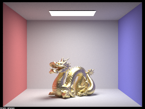
Below is a sequence of 4 images of CBdragon_microfacet_au.dae with alpha set to 0.005, 0.05, 0.25, and 0.5. All images use 1024 samples/pixel (lower sampling rates leave many bright noise spots throughout the image), 1 sample per light, and 5 maximum bounces. When alpha is very small, the dragon approaches perfect mirror reflection. As alpha increases, the dragon becomes rougher - i.e. there is greater variation among microfacet normals. The dragon appears more diffuse (less glossy and reflective). With fewer reflections, the image overall also becomes less susceptible to the bright noise spots.

alpha = 0.005
|

alpha = 0.05
|
alpha = 0.25
|

alpha = 0.5
|
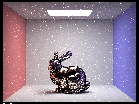
Below are two images of CBbunny_microfacet_cu.dae rendered with cosine hemisphere sampling and importance sampling. Both images use 64 samples per pixel, 1 sample per light, and 5 maximum bounces. Cosine hemisphere sampling is more inefficient, sampling uniformly regardless of lighting information, and takes longer to converge; for the same parameters, it appears noisier. Additionally, for this dae, cosine hemisphere sampling overly accentuates dark areas of the bunny and thus seems particularly insuitable for this BRDF.
|

|
Below is an image of CBdragon_microfacet_au.dae with eta and k parameters replaced to represent silicon. I used alpha = 0.05 to make the dragon glossy (more like a polished silicon wafer). I used 1024 samples/pixel, 1 sample per light, and 5 maximum bounces. I found the following parameters on https://refractiveindex.info at wavelengths 614 nm (for red), 549 nm (for green), and 466 nm (for blue):
| Color | eta |
k |
| Red | 3.9186 | 0.023600 |
| Green | 4.0903 | 0.041535 |
| Blue | 4.5288 | 0.11463 |

|
Part 4: Depth of Field
In the pinhole camera model that we used in Assignment 3 up to this part, each ray forms a straight line between the image plane and the scene, traveling through a single fixed "pinhole" on the z=0 plane in camera space. This results in each point of the scene being rendered at exactly one point on the image plane, so everything appears in focus. In a thin-lens camera model, each point on the image plane receives radiance from a "cone" of rays that intersect anywhere on the lens. There is one focal plane in the scene at which rays from a single point on that plane hit the lens and refract to focus on a single point on the image plane - i.e. objects at this plane are "in focus."" For points on planes in the scene in front of or behind this focal plane, the rays enter the lens, refract, and focus on points that lie in front of or behind the image plane. This results in a circle of confusion, or blur, on the image plane itself. By modeling our lens in this slightly more realistic way, we can achieve a depth of field effect that can be modulated by changing the lens radius (aperture) and focal distance of our camera.
In this part, we implement the Camera::generate_ray_for_thin_lens() function. It is based on Code::generate_ray() but additionally takes in 2 random polar coordinates to uniformly sample the thin lens. The function defines the rays shown in the diagram below (from the assignment spec) and returns the blue ray:

|
The red ray is simply the generated ray from our original generate_ray() function with a z-direction of -1. The direction of the blue ray in camera coordinates is found as the normalized direction from pLens, the sample point on the lens corresponding to the random inputs rndR and rndTheta, to pFocus, the point in focus on the focal plane in the scene at z = -focalDistance. pLens is found by converting rndR and rndTheta to Cartesian coordinates and scaling by the lens radius - i.e. pLens=(lensRadius √rndR⋅cos(rndTheta),lensRadius √rndR⋅sin(rndTheta),0) (as given in the asssignment spec). pFocus is simply found as the direction of the red ray multiplied by t_intersect, the time of the red ray's intersection with the focal plane, which is simply focalDistance (or more explicitly, [intersection_z = redray_origin_z + redray_direction_z * t_intersect => -focalDistance = 0 + (-1) * t_intersect)). The blue ray is then generated by setting the ray's origin to pLens in world coordinates (by applying the c2w matrix) with a pos offset and the direction as found before, also converted to world coordinates with c2w.
Below is a "focus stack" where I focus at 4 visibly different depths through the CBdragon_microfacet_au.dae scene. I used a fixed lens radius of 0.2 for all images and changed the focal distance to 4.5, 4.7, 4.9, and 5.1, corresponding roughly to focal planes from the head of the dragon to its tail.
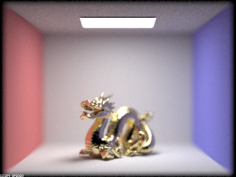
CBdragon_microfacet_au.dae, focal distance = 4.5
|
CBdragon_microfacet_au.dae, focal distance = 4.7
|

CBdragon_microfacet_au.dae, focal distance = 4.9
|

CBdragon_microfacet_au.dae, focal distance = 5.1
|
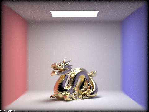
Below is a sequence of 4 pictures with visibly different aperture sizes (0, 0.2, 0.4, and 0.6), all with focal distance of 4.5 (the front tip of the dragon). When the lens radius is 0 (pinhole camera), the field of view is quite large, and the entire image appears in focus. As the lens radius increases, the field of view becomes increasingly small, until for a lens radius of 0.6, the entire image is blurry except a very thin plane that only a sliver of the dragon's nose lies on.
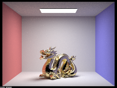
CBdragon_microfacet_au.dae, lens radius = 0
|
CBdragon_microfacet_au.dae, lens radius = 0.2
|
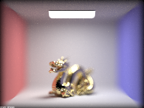
CBdragon_microfacet_au.dae, lens radius = 0.4
|
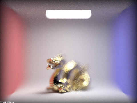
CBdragon_microfacet_au.dae, lens radius = 0.6
|