Overview
This project goes through the basic building blocks of simulating scenes with actual physics-based constraints. We start by modeling a cloth as a network of masses connected by springs and applying first-order forces to those. We then implement Verlet integration to simulate the cloth's movement across a series of time steps, making sure that the cloth does not pass through other objects or itself. Finally, this project also implements various shaders that run on GPU to yield stunning graphics effects in real-time. The hardest parts of this for me were wrapping my head around hashing for efficient self-collision checks, getting used to the syntax of GLSL, and also tweaking the parameters of the shaders to achieve a better look. Luckily, this project didn't take as long to render as the last, but refining all the open-ended constants and re-running simulations each time did end up taking a good amount of time.
Part I: Masses and springs
In this part, a grid of masses and springs is constructed in Cloth::buildGrid(). The positions of the masses are distributed such that num_width_points masses span the grid's width and num_height_points masses span the grid's height. In our 3D coordinate system, the grid's width is distributed along the x-axis. If the cloth's orientation is HORIZONTAL, the y-coordinate for all masses = 1, and the grid's height is distributed along the z-axis. If the cloth's orentation is VERTICAL, the z-coordinate for each mass is assigned a random offset between -1/1000 and 1/1000, and the grid's height is distributed along the y-axis. For each mass, the Cloth's pinned vector is traversed, and if that mass's width and height index is found in pinned, then the PointMass's pinned variable is set to true to indicate that that mass should be pinned in place during simulation.
Springs are constructed by iterating through each mass. For each mass that has a mass to its left (every mass except the last row), a structural spring between that mass and the one to its left is added. For each mass that has a mass above it (every mass except the last column), a structural spring between that mass and the one above it is added. For each mass that has a mass diagonally above and to the left (every mass except the last one in the upper-left corner), a shearing spring between that mass and the one diagonally above and to the left is added. For each mass that has a mass diagonally above and to the right (every mass except the one in the upper-right corner), a shearing spring between that mass and the one diagonally above and to the right is added. For each mass that has 2 masses to the left (every mass except the ones in the second-to-last and last rows), a bending spring between that mass and the one two over to the left is added. Finally, for each mass that has 2 masses above it (every mass except the ones in the second-to-last and last columns), a bending spring between that mass and the one two above it is added.
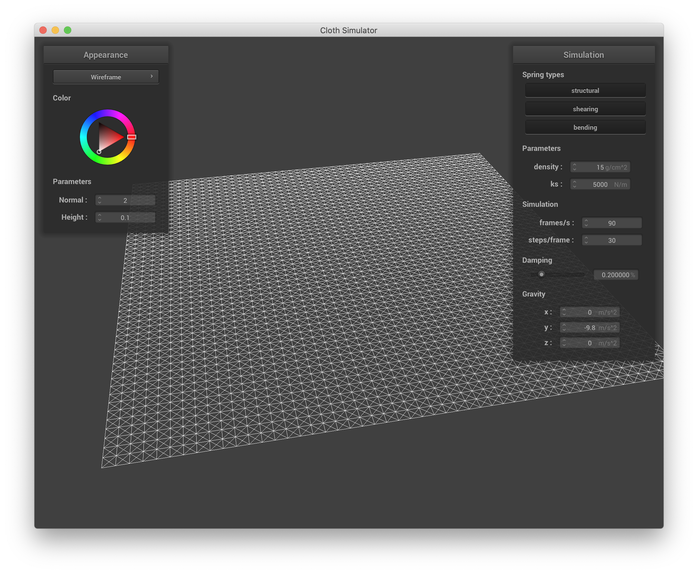
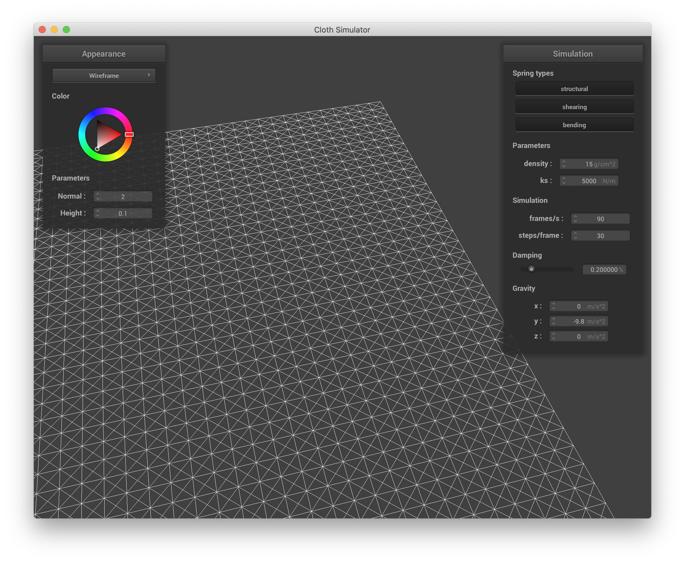
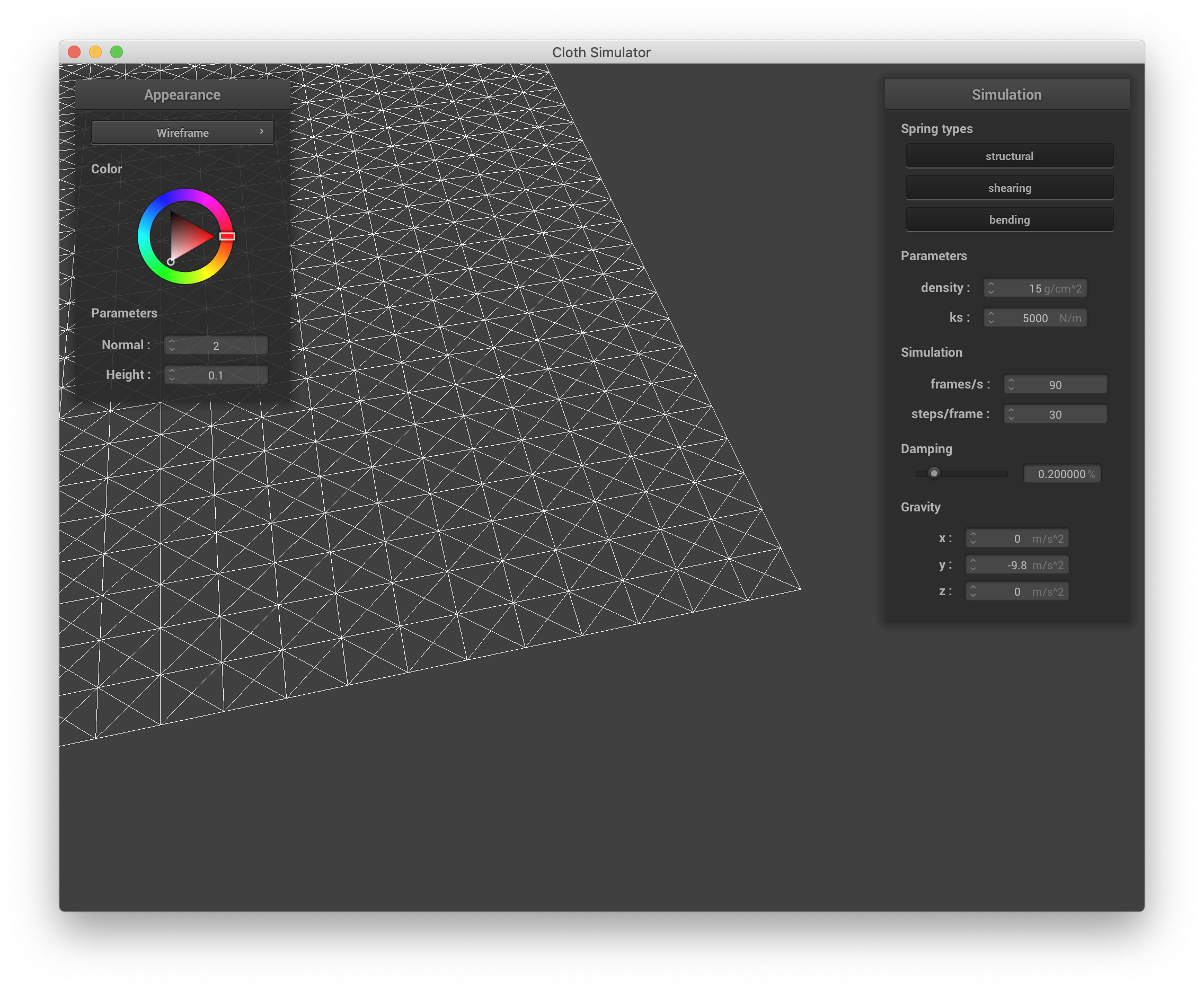
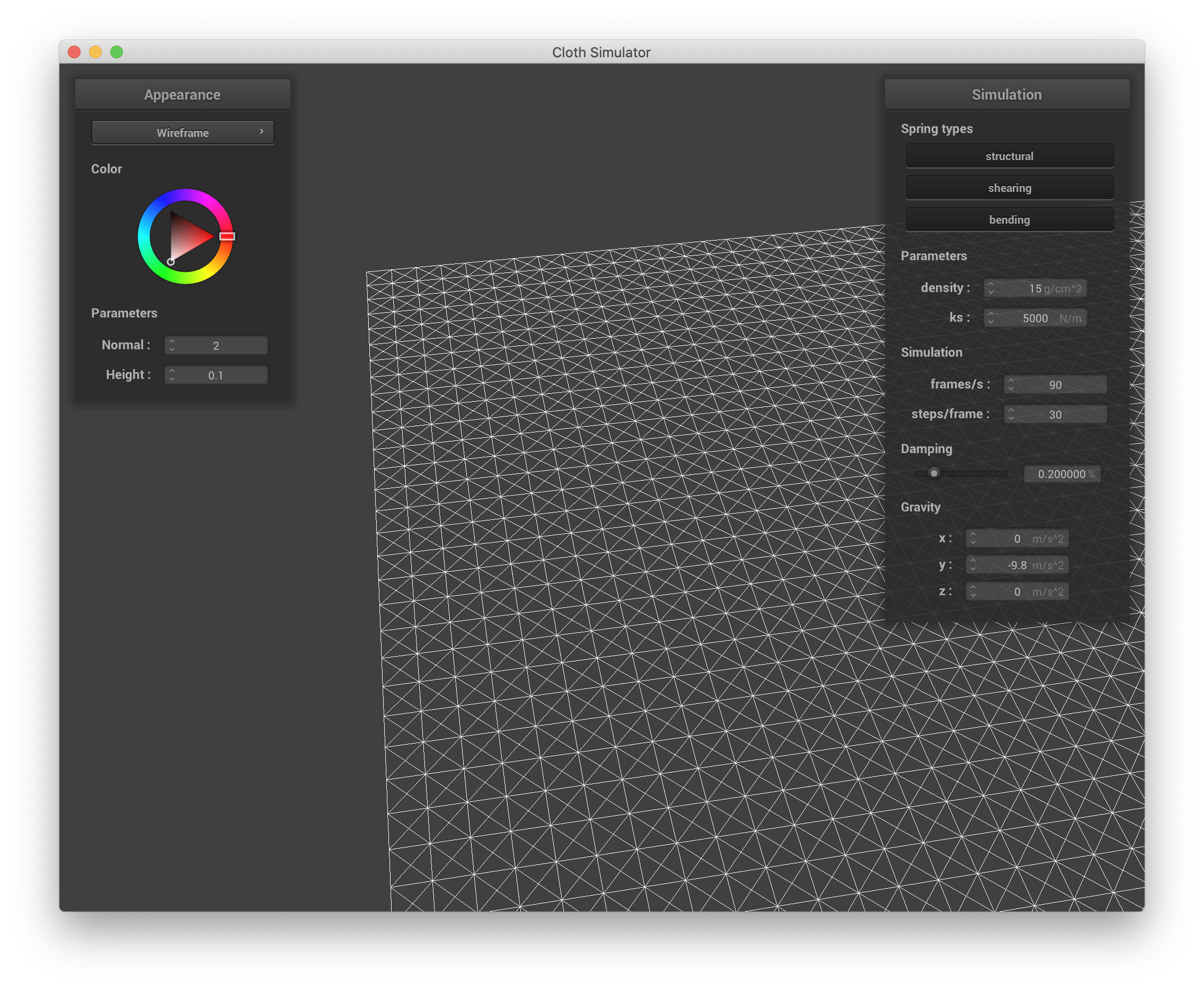
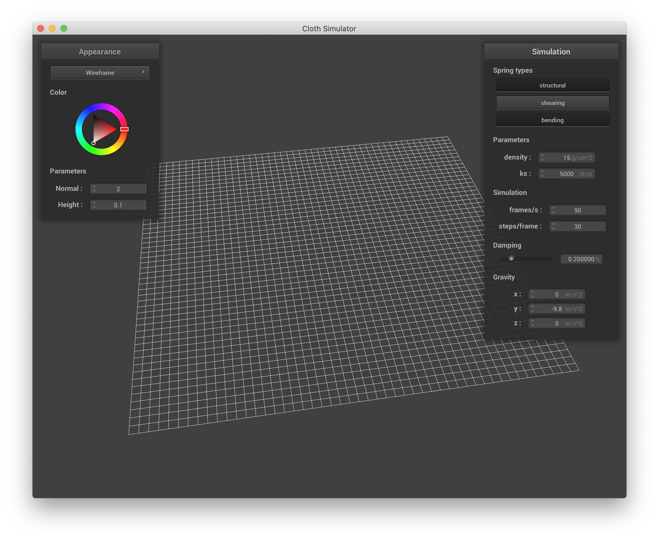
Below are screenshots of scene/pinned2.json illustrating the cloth wireframe and the structure of its point masses and springs.
|
|
|
|
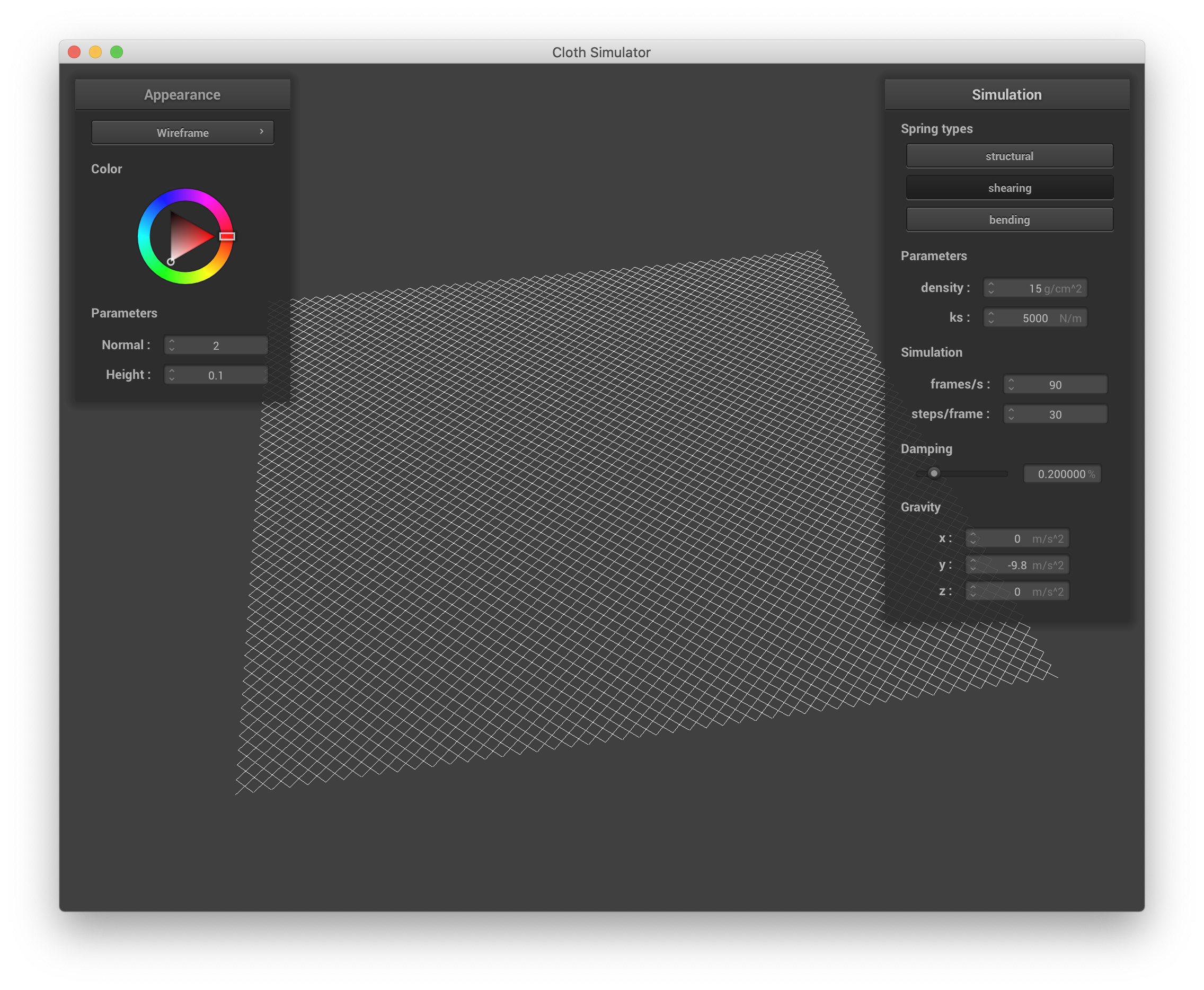
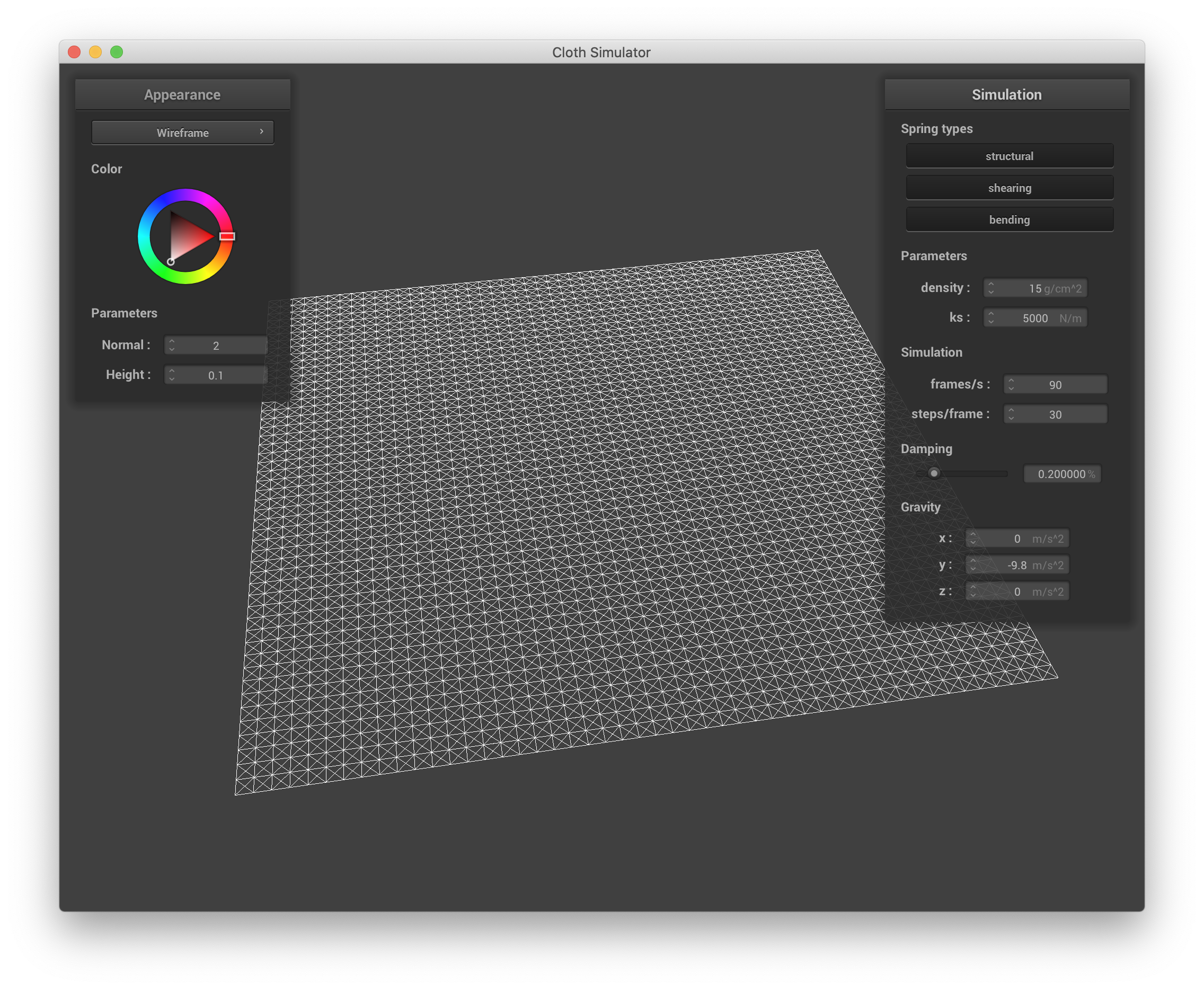
Below are screenshots showing what the wireframe looks like without shearing constraints, with only shearing constraints, and with all 3 constraints.
|
|
|
Part II: Simulation via numerical integration
To be able to simulate the cloth's movement across time, Verlet integration is used between each time step in Cloth::simulate(). First, any existing forces stored in each PointMass's forces variable are cleared, and forces acting on each point mass at the current time step are calculated. There is a net external force that is simply the sum of the accelerations in external_accelerations times the mass property of the cloth (F=ma). There are also spring forces whose magnitude is the spring constant ks multiplied by the displacement of the spring (for simplicity, we assume the same ks, found in the cloth's parameters cp, for all springs, except bending springs use a spring constant = 0.2 * ks). The displacement of the spring is the distance between the 2 masses on either end of the spring minus the spring's rest length. For the 2 point masses attached to each spring, the resulting spring force is multiplied by the normalized direction vector from one point mass to the other and added to that point mass's forces variable.
Verlet integration is an explicit integrator that estimates each unpinned point mass's new position at time t + dt as x_t + v_t*dt + a_t * dt^2. We further estimate the current velocity, v_t, as x_t - x_(t-dt), or the difference between the current position and the previous one. a_t is the current acceleration that is simply the total forces on that point mass divided by the mass variable. To simulate loss of energy (friction, heat loss, etc.), we add a simply damping term to obtain the final estimator, x_(t+dt) = x_t + (1 - damping/100) * (x_t - x_(t-dt)) + a_t * dt^2. The positions of pinned masses are left untouched.
To prevent the cloth from falling through the scene to infinity and unrealistically stretching from its pinned points, we constrain the changes such that each spring does not stretch beyond 10% of its rest_length. At the end of each time step, we iterate through each spring, and if the distance between the 2 point masses on either side of the spring is greater than 1.1 * rest_length, we calculate the total correction distance that the masses must be moved toward one another such that they are only separated by 1.1 * rest_length. If one of the masses is pinned, the unpinned mass's position is updated by adding the correction distance along the vector pointing from it to the pinned mass. If both masses are unpinned, each mass moves half of the correction distance along the vector pointing from it to its partner. If both masses are pinned, nothing is done, but these masses shouldn't have been moved in the first place anyway.
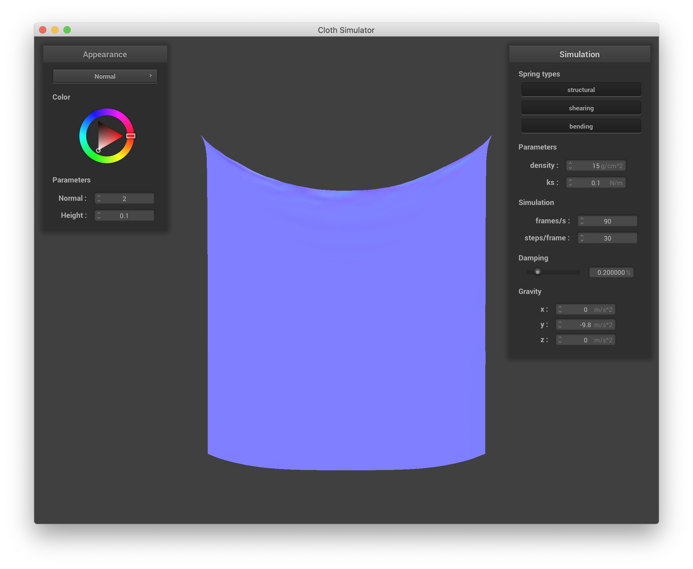
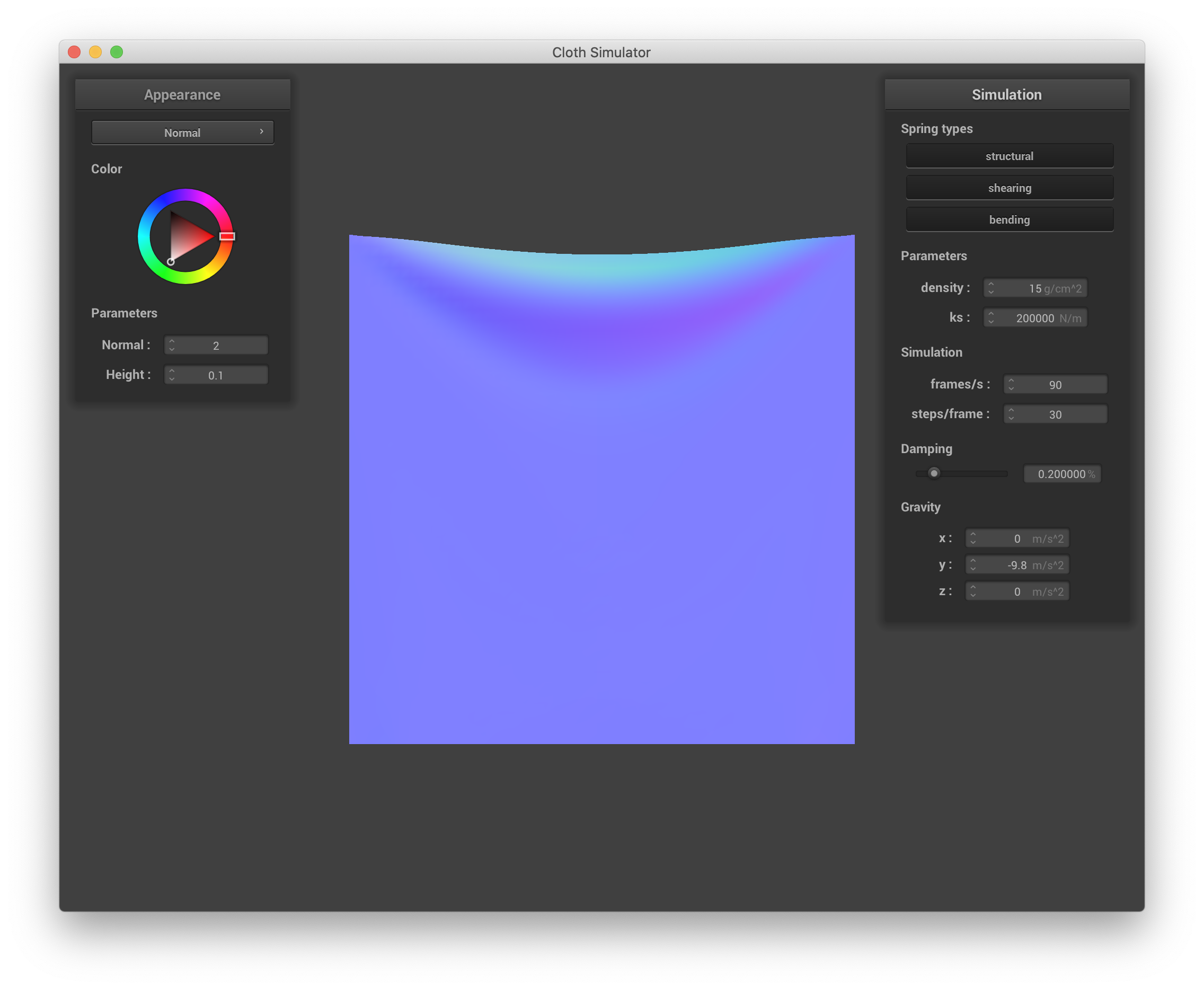
Changing ks changes the "bounciness" of the cloth on the scale of individual masses/springs, altering both the final state of the cloth and the dynamics of how that state is reached. With a very low ks, the cloth exhibits much more jittering and shimmering and takes a much longer time to settle. When it does settle, it sags more. With a very high ks, the point masses are essentially connected by much stiffer springs that require greater forces to displace, so there are fewer "fine" bounces as the cloth moves towards its resting state, which is also much less saggy. Below are screenshots with ks = 0.1 N/m and ks = 200000 N/m approximately 3 seconds after starting the simulation and then 10 seconds after that illustrate this behavior.
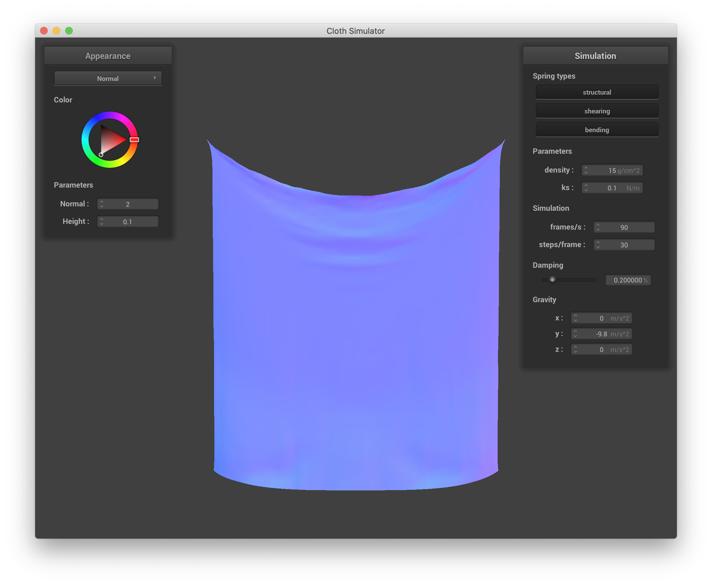
ks = 0.1, ~3 s into simulation |
ks = 0.1, ~10 s into simulation |

ks = 200000, ~3 s into simulation |
ks = 200000, ~10 s into simulation |
Changing density changes both the final resting state of the cloth and the dynamics of how that state is reached. Increasing density increases the mass of each point mass. When density is very small, the point masses are very light and hardly displace the springs that connect them, and the cloth appears to "float" gently to its final position, which is much less sagged than with the default parameters (similar to the effect of high ks). When the density is very high, the cloth appears to fall much more heavily as each spring is stretched more (similar to the effect of low ks). The final resting state is much more sagged than with the default parameters, and the cloth doesn't actually appear to entirely settle at all, instead continuing to bounce and shimmer where the springs are most obviously stretched (the top edge). Below are screenshots of the cloth's state after ~10 seconds with density set to 0.5 g/cm^2 and 100000 g/cm^2.
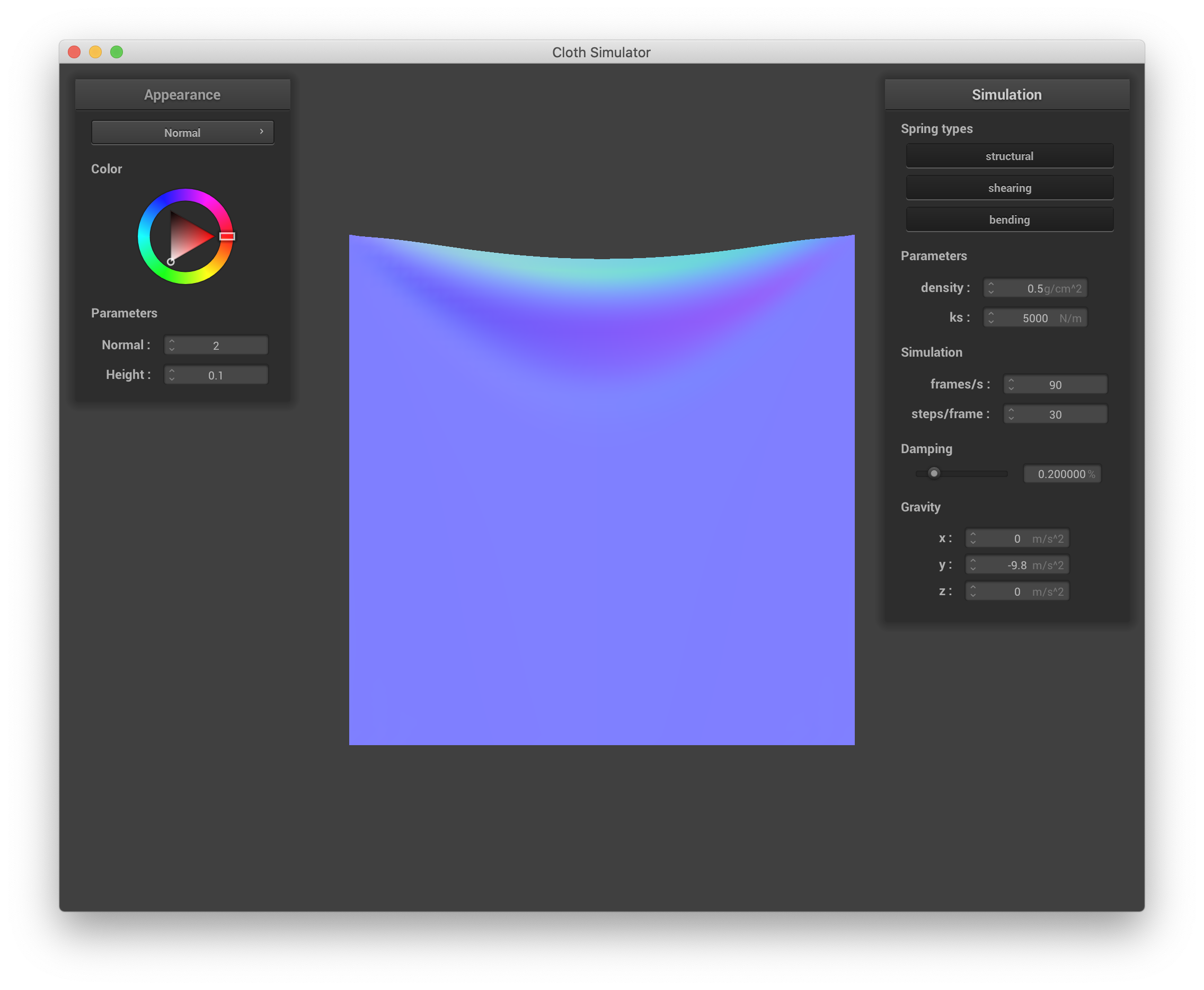
|
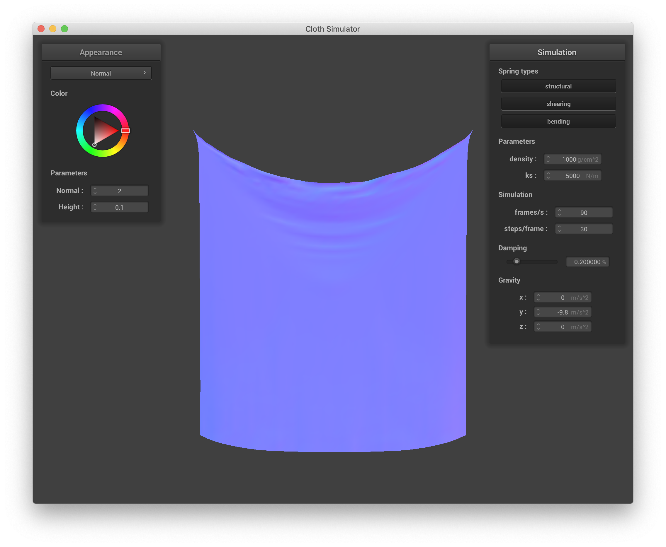
|
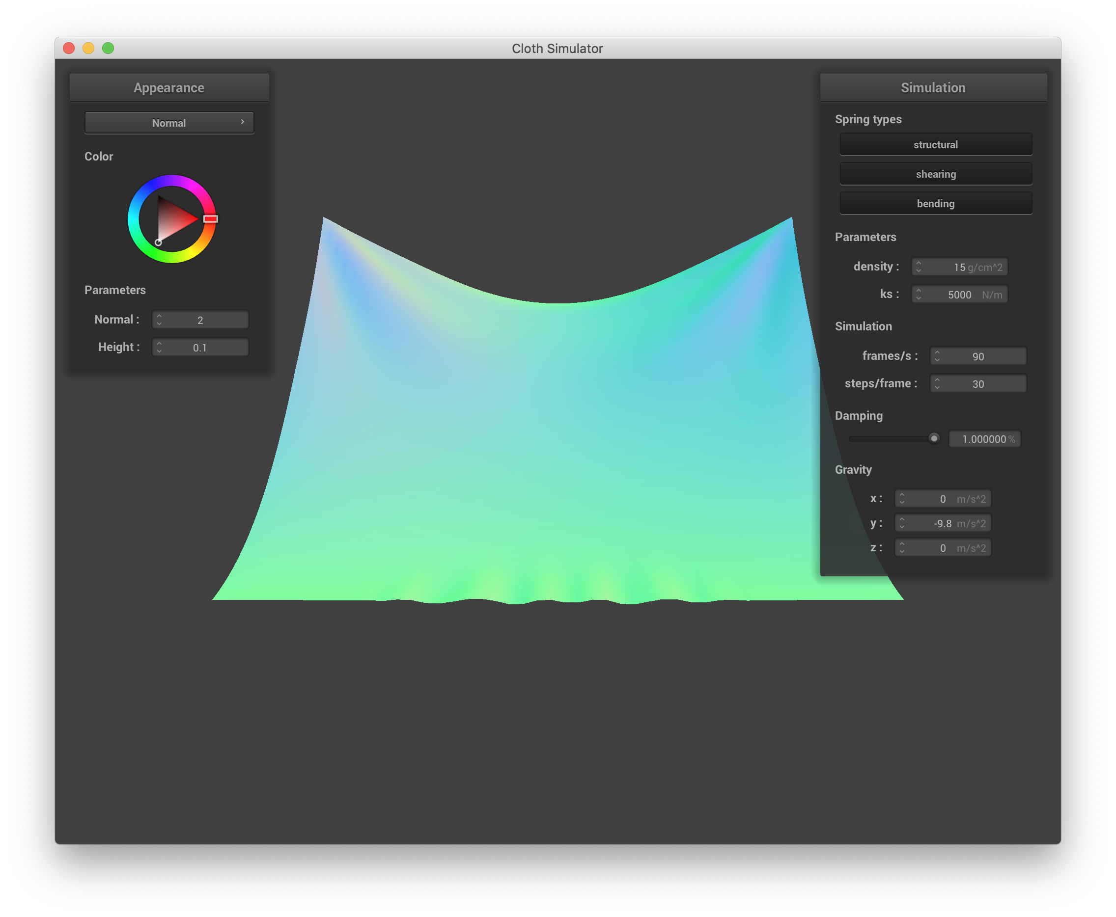
Finally, changing damping affects the bounciness (both on a point mass/spring scale and the "macroscale") of the cloth and how quickly the cloth settles into its final resting state. However, this final resting state itself is the same as the resting state with default parameters. When damping is set very low (in the extreme case, to 0%), the cloth continues waving and bouncing up and down with large magnitudes for a long time, as illustrate by the 4 below screenshots at sequential time steps across ~30 seconds:

|
|
|
|

|
|

|
|
Below is a screenshot of scene/pinned4.json in its final resting state:

scene/pinned4.json, default parameters |
Part III: Handling collisions with other objects
In this part, collisions with spheres and planes are implemented in the respective collision() functions of the Sphere and Plane classes. For a sphere, a point mass is determined to lie on or inside the sphere if the magnitude of the vector d between the sphere's origin and the point mass's position is less than or equal to the sphere radius. If this is the case, a tangent point is calculated as the sphere's origin plus a vector with magnitude radius and direction equal to the normalized d vector. A correction vector needed to bump the point mass to the surface of the sphere is calculated as the vector from the point mass's last_position to the tangent point. Finally, the point mass's position variable is updated to be the last_position plus this correction vector, which is scaled down slightly due to friction with the constant (1 - friction). Similarly, for a plane, a point mass is determined to collide with the plane if it crosses from one side to the other from the last time step to the current - i.e. the dot product between the plane's normal vector and the vector from the plane's point to the mass's last_position is opposite in sign to the dot product between the normal vector and the vector from point to the mass's position (or one/both are zero). If this is the case, the tangent point where the point mass should have intersected the plane is calculated as the mass's position minus the projection of the vector from the plane's point to the mass's position onto the plane's normal. The correction vector is the vector from the point mass's last_position to this tangent point. It is offset by SURFACE_OFFSET along the plane's normal such that last_position plus the correction results in a position on the same side of the plane as last_position. Finally, as with the sphere, the mass's position is updated as last_position plus this correction vector, dampened by a (1-friction) term.
The Cloth's simulation() function is also updated. For each point mass, we iterate through the input vector collision_objects, and for each CollisionObject, collide() is called with an input of the current point mass.
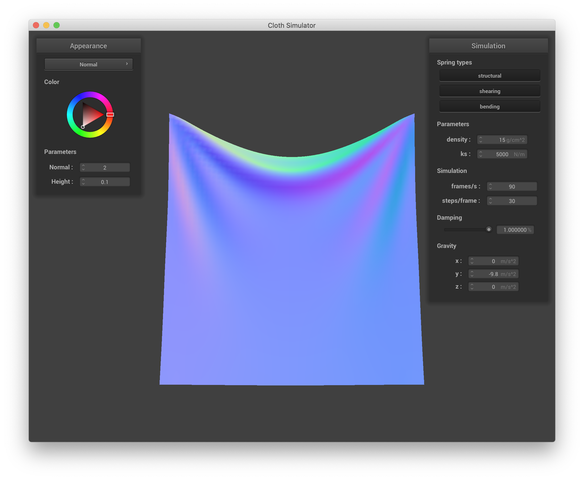
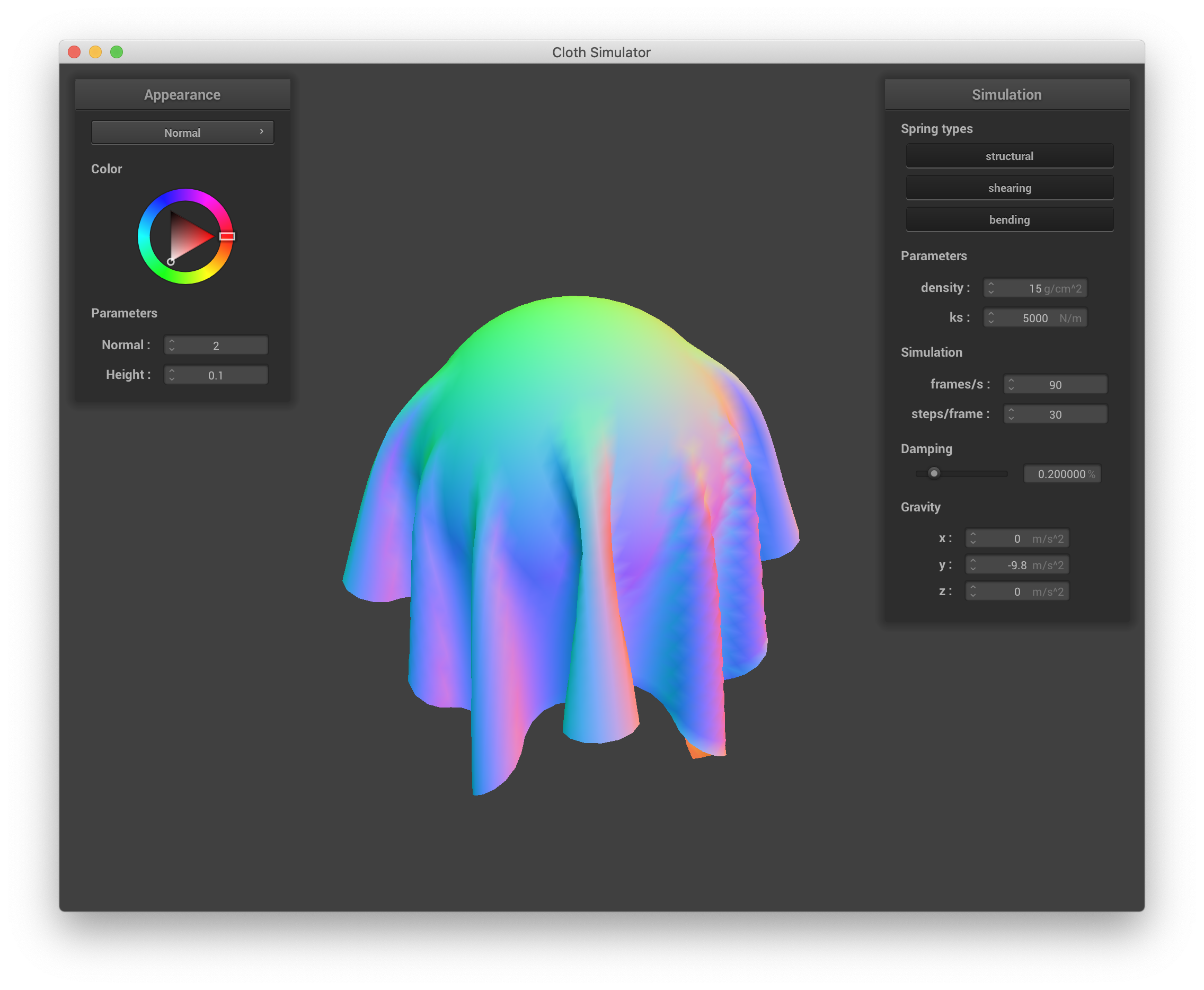
Below are screenshots of the shaded cloth from scene/sphere.json in its final resting state using the default ks = 5000, as well as with ks = 500 and ks = 50000. All other parameters are left as their defaults. As discussed in the last section, as ks increases, the cloth becomes stiffer. When ks is small (=500 N/m), we see that the cloth conforms well to the sphere, making the shape of the underlying sphere very obvious. As a result, there are also more fine ruffles in the part of the cloth that drapes down from the sphere. When ks is large (=50000 N/m), the cloth is too stiff to fully conform to the sphere, so the underlying shape of the sphere is less apparent. Additionally, the ruffles from the draped part of the cloth are fewer and larger.
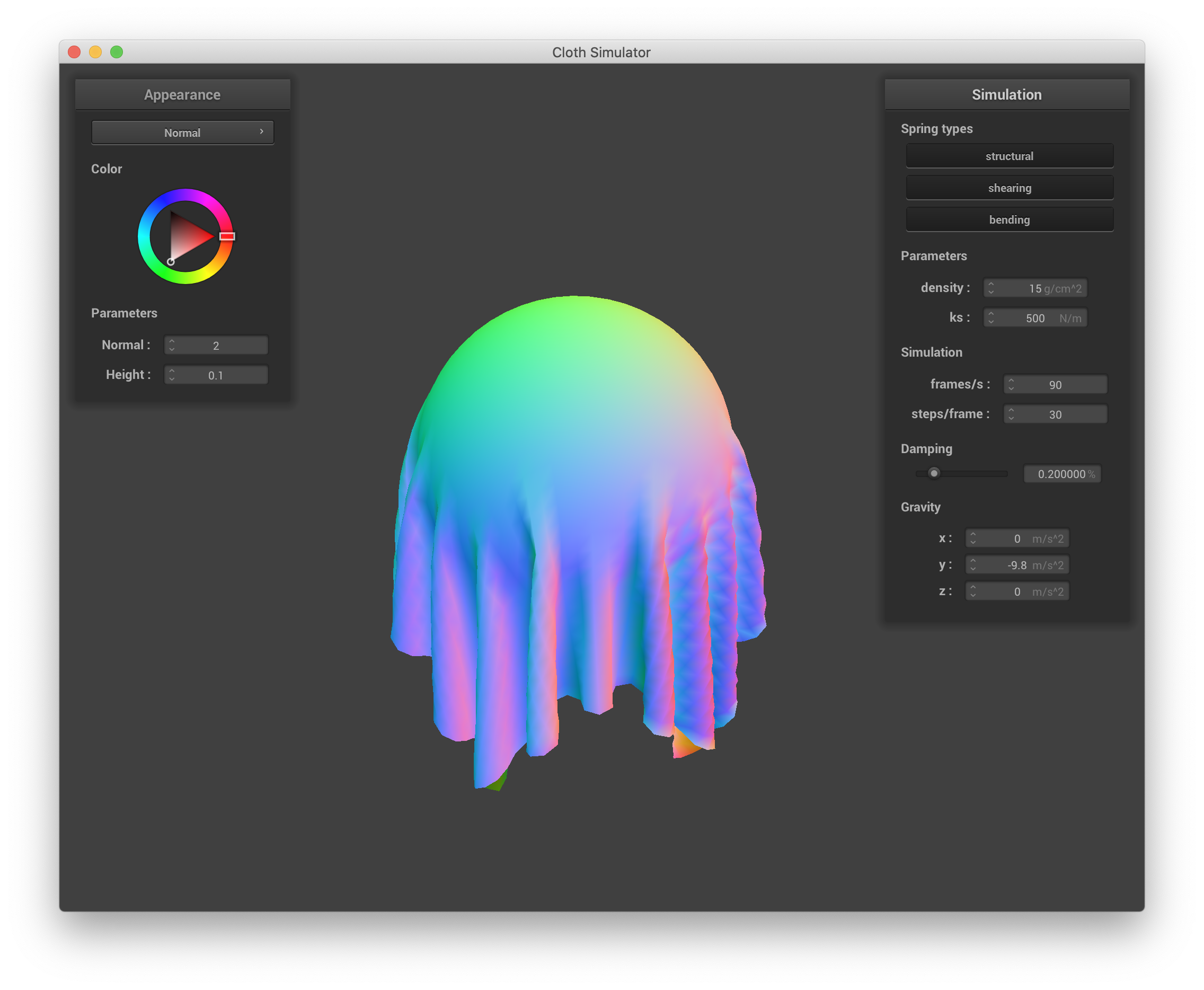
ks = 500 |
ks = 5000 (default) |

ks = 50000 |
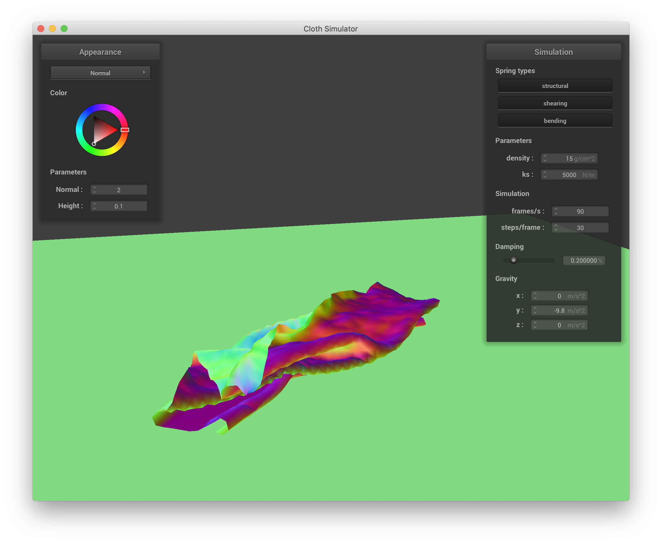
Below is a screenshot of a resting cloth on a plane after simulating scene/plane.json.

|
Part IV: Handling self-collisions
In this part, spatial hashing is used to handle self-collisions without the expensive O(n^2) operation of looping through and potentially updating the forces of all pairs of point masses. This is done by first mapping each point mass's position to a float that uniquely represents a 3D box volume. As suggested by the assignment spec, the 3D space is divided into 3D boxes with dimensions (w = 3 * width / num_width_points, h = 3 * height / num_height_points, max(w,h)). A point mass's position is then truncated to the box that it lies. Next, a unique identifier for this box is calculated. I seem to be a little rusty/lacking understanding of the math of hash tables, but prime numbers as coefficients for a linear combination of the x, y, and z indices of the 3D boxes seemed to work (I used 17, 23, and 29, respectively) for this application. While I didn't take the time to see if this truly guarantees a unique identifier for each 3D box, intuitively, we don't want to use a hash function that returns numbers that quickly blow up (and eventually result in numerical errors), but we also want the identifiers to be fairly well-spaced.
simulation() function is updated to build a spatial map by calling build_spatial_map(), which iterates through all point masses, adds their hash to the cloth's map if it doesn't already exist, and adds the point mass to the appropriate hash index in the map. Next, we iterate through all point masses and check for self-collision by calling self_collide(). self_collide() takes a PointMass as input and checks its distance to every other candidate point that shares its hash position, as determined by the Cloth's map. If the distance is not zero (i.e. we don't check a mass against itself) and is less than 2 * thickness, the input point mass must be moved because it is basically colliding with the candidate point mass. A correction vector in the opposite direction from the point mass to the candidate point with magnitude 2 * thickness - distance is added to a running total correction vector. After looping through all candidate point masses, the total correction vector is averaged by dividing by the total number of correction vectors and additionally dividing by the number of simulation steps before finally being added to the input point mass's position.
Below are a series of screenshots showing how the cloth in selfCollision.json falls and folds on itself:

|

|
|
|
|
|
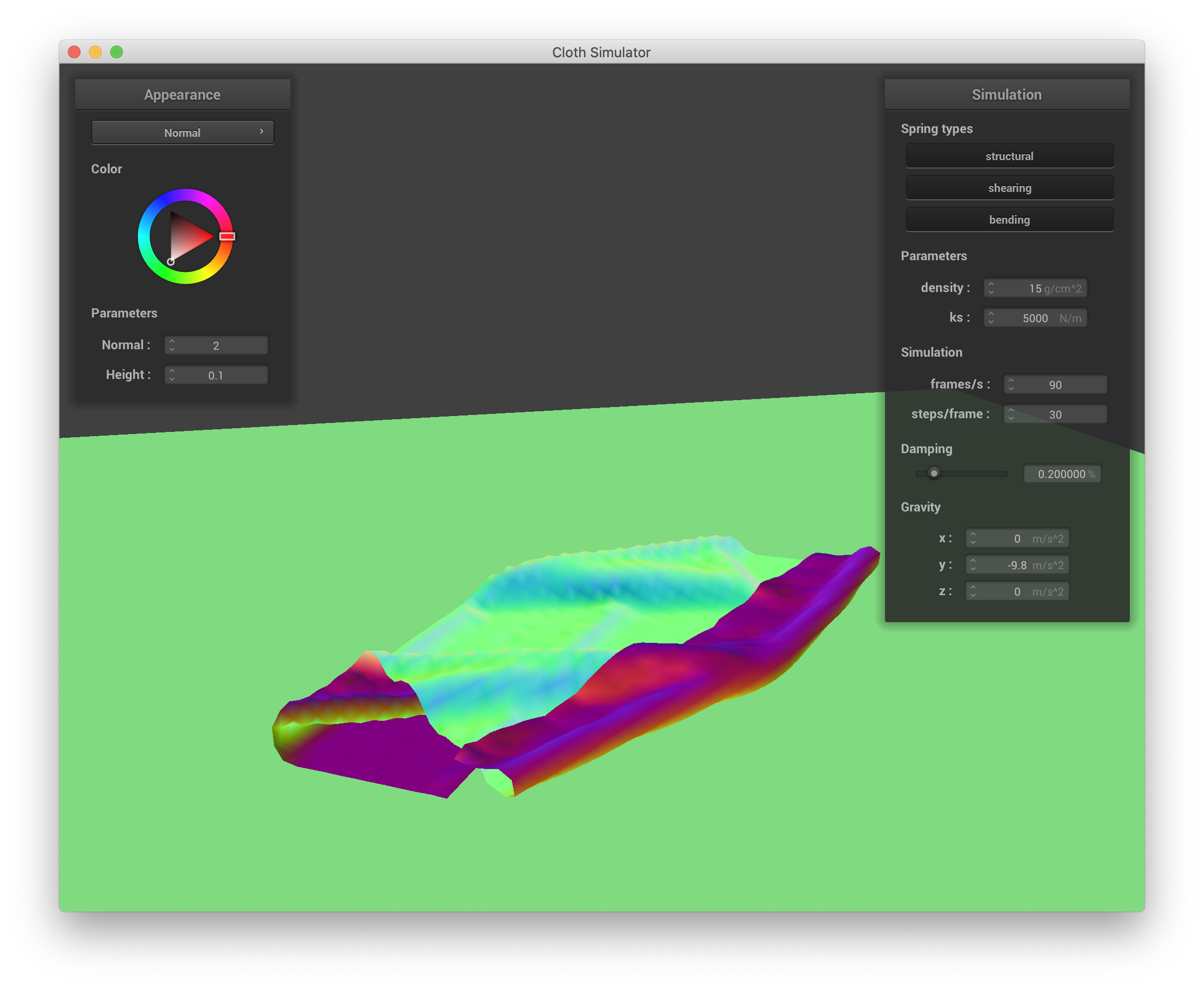
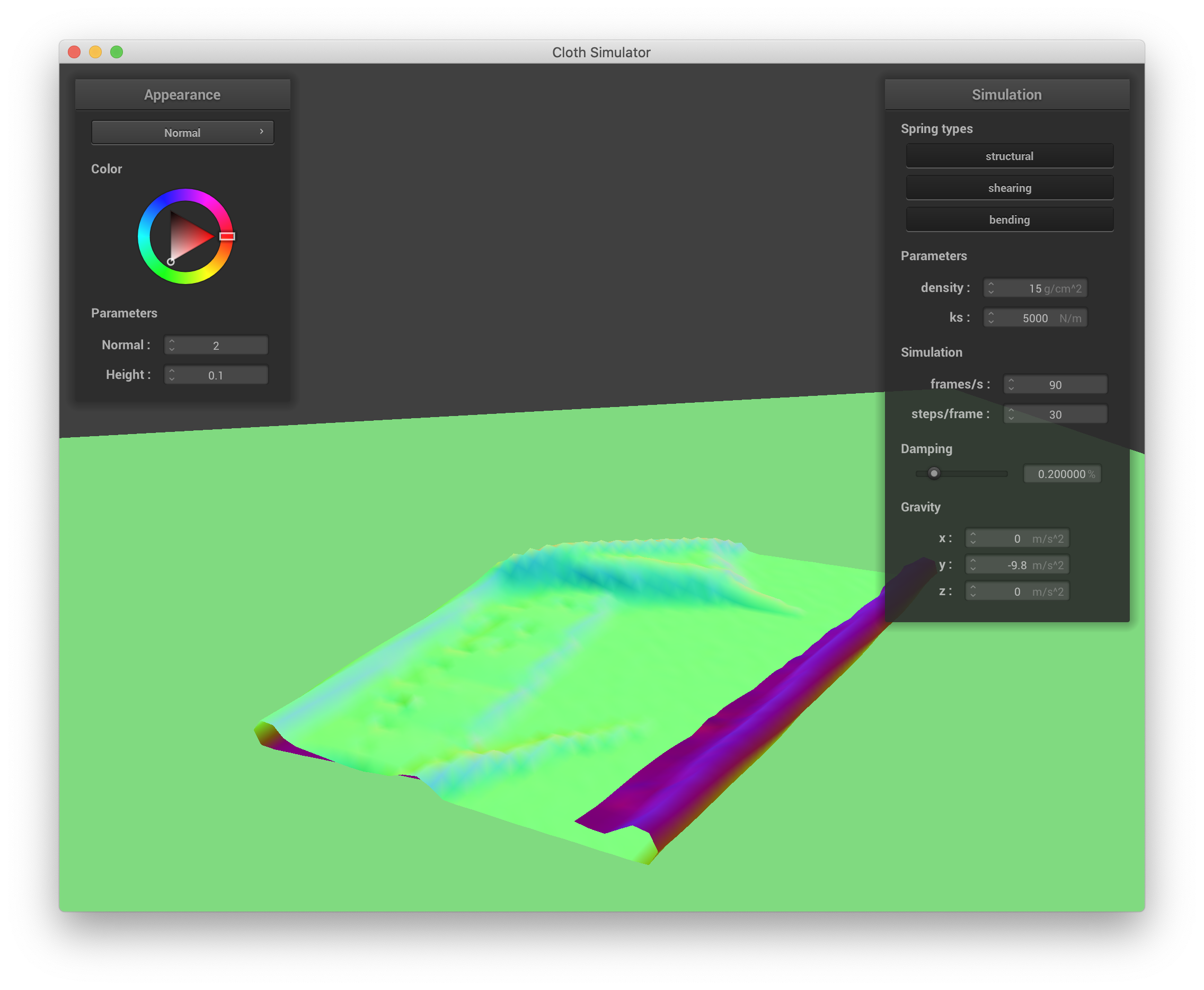
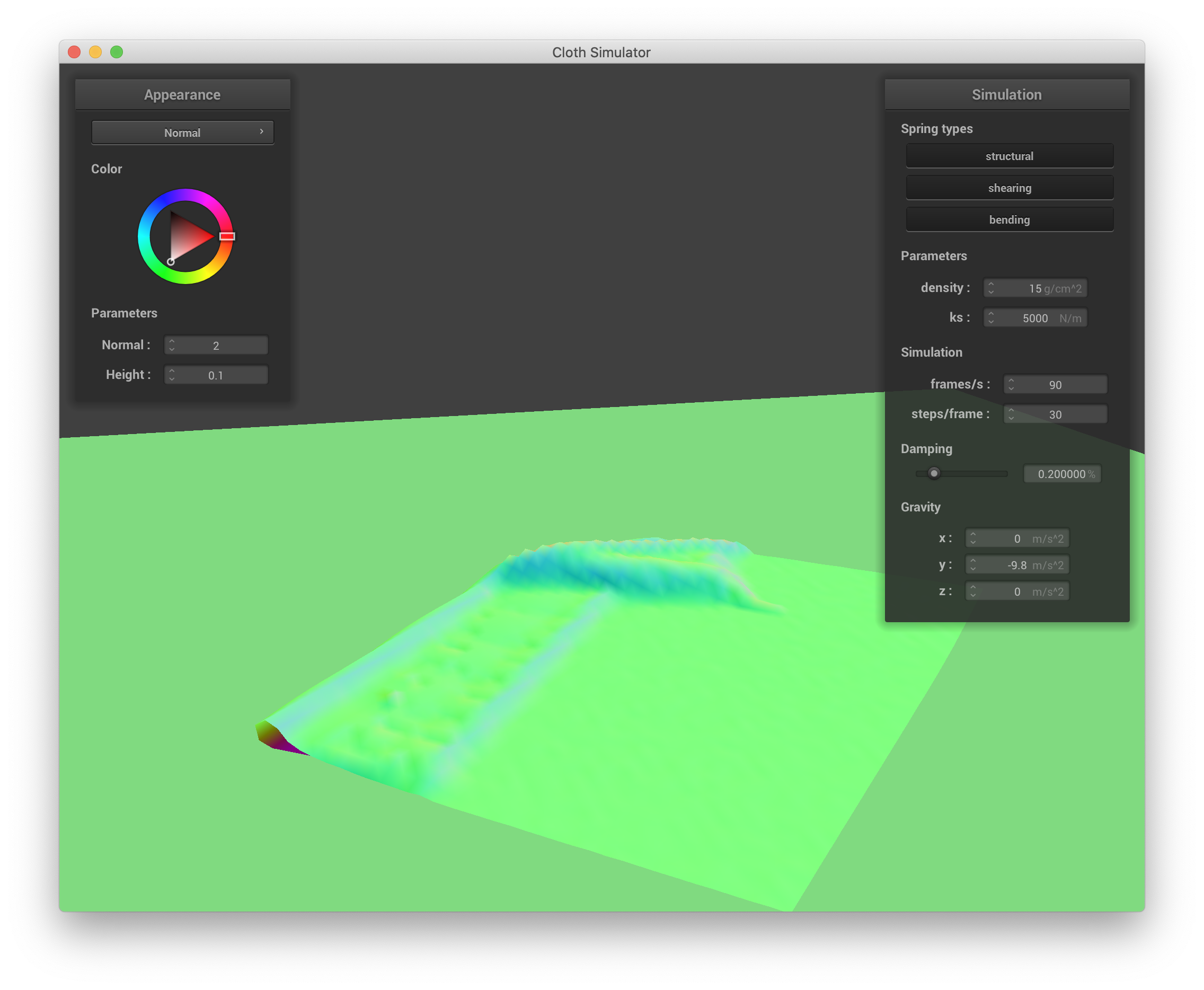
Varying density changes how quickly and "ruffley" the cloth falls to the ground and settles. When the density is small, the cloth appears to more gently float to the ground, exhibiting larger, smoother folds. Below are screenshots of lowering density to 1 g/cm^3:
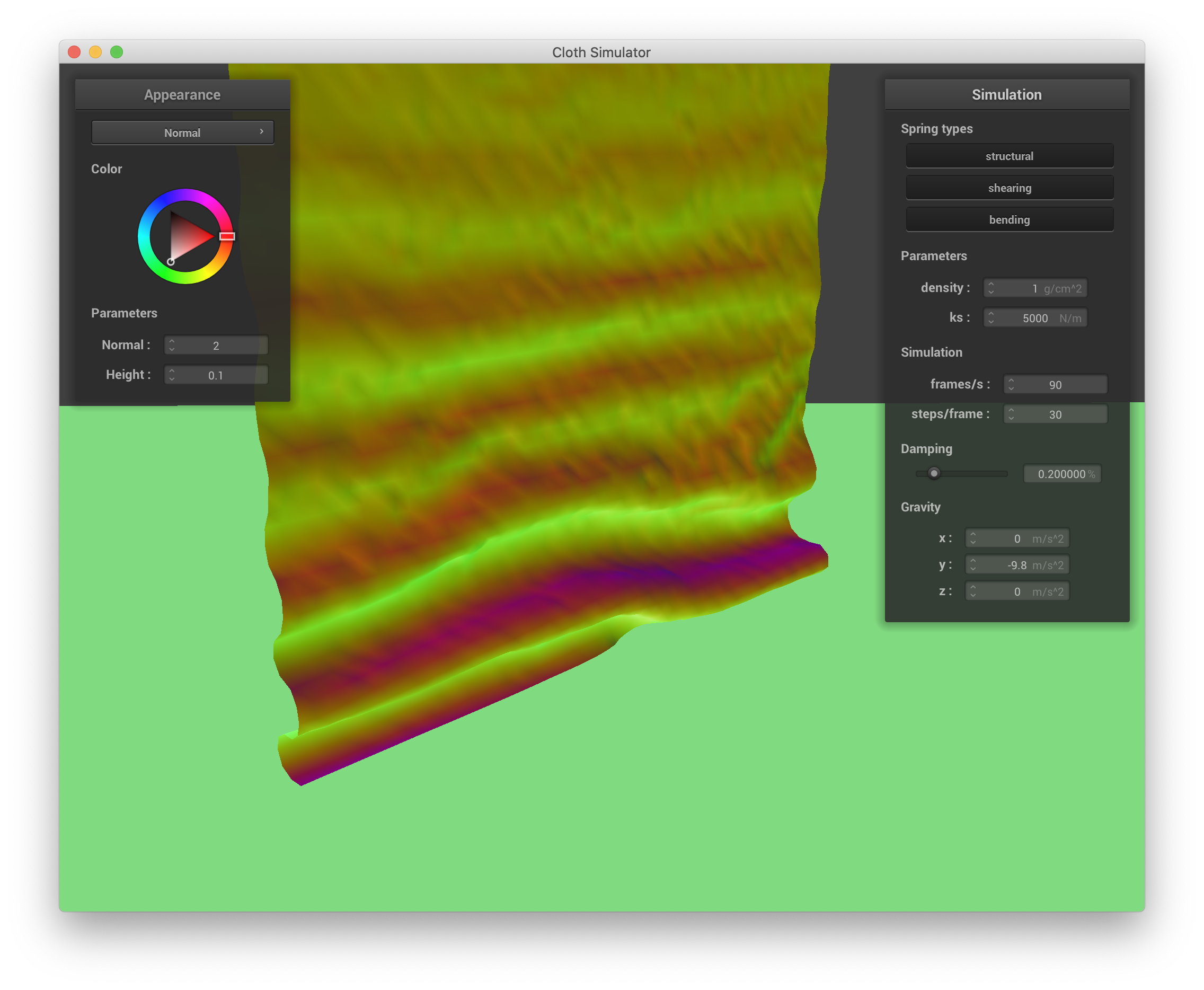
|
|
|
|
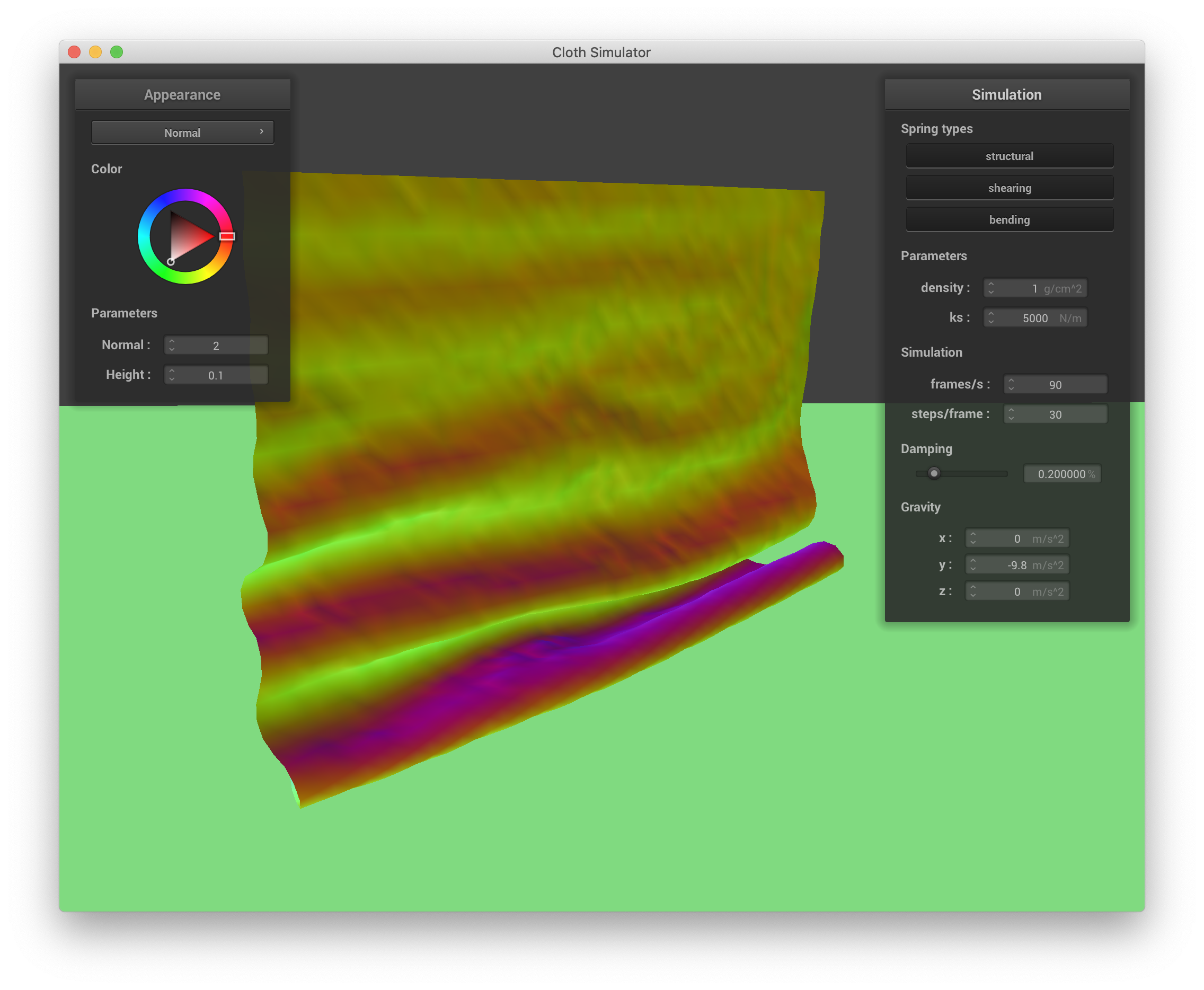
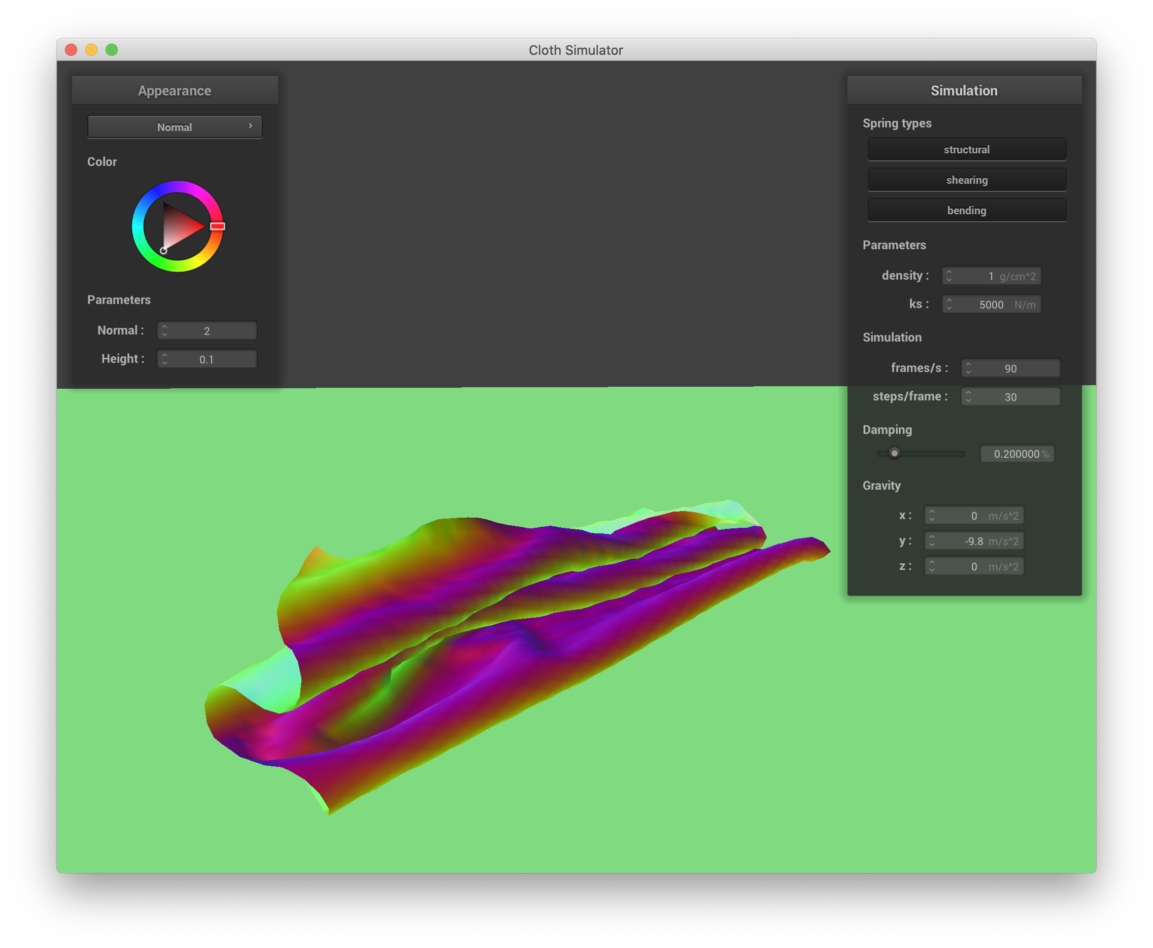
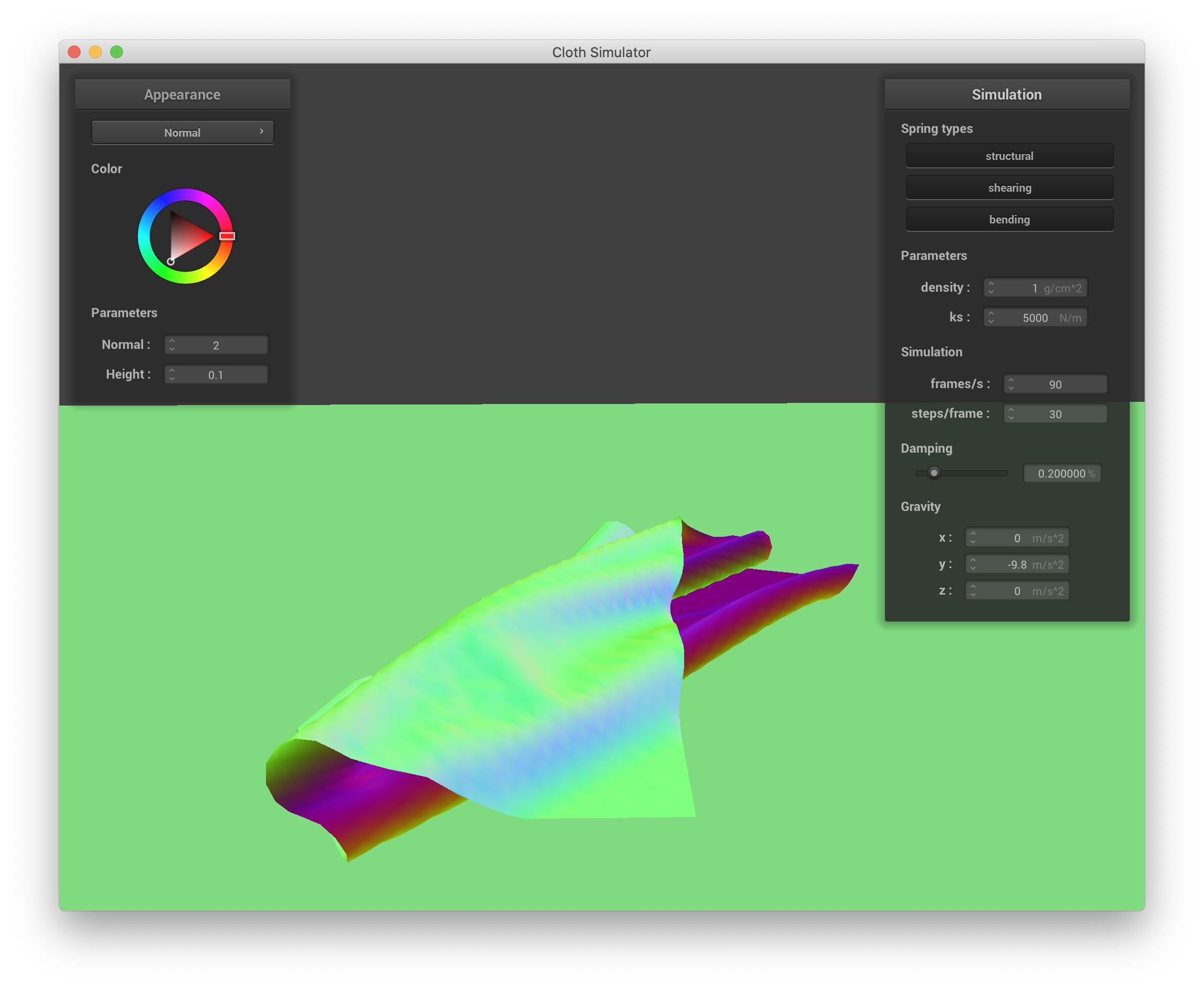
Conversely, increasing density causes the cloth to tend to fall and crumple on top of itself more, creating much higher-frequency ruffles and more self-collisions. Below are screenshots of simulating the cloth with a density of 100 g/cm^3:

|

|
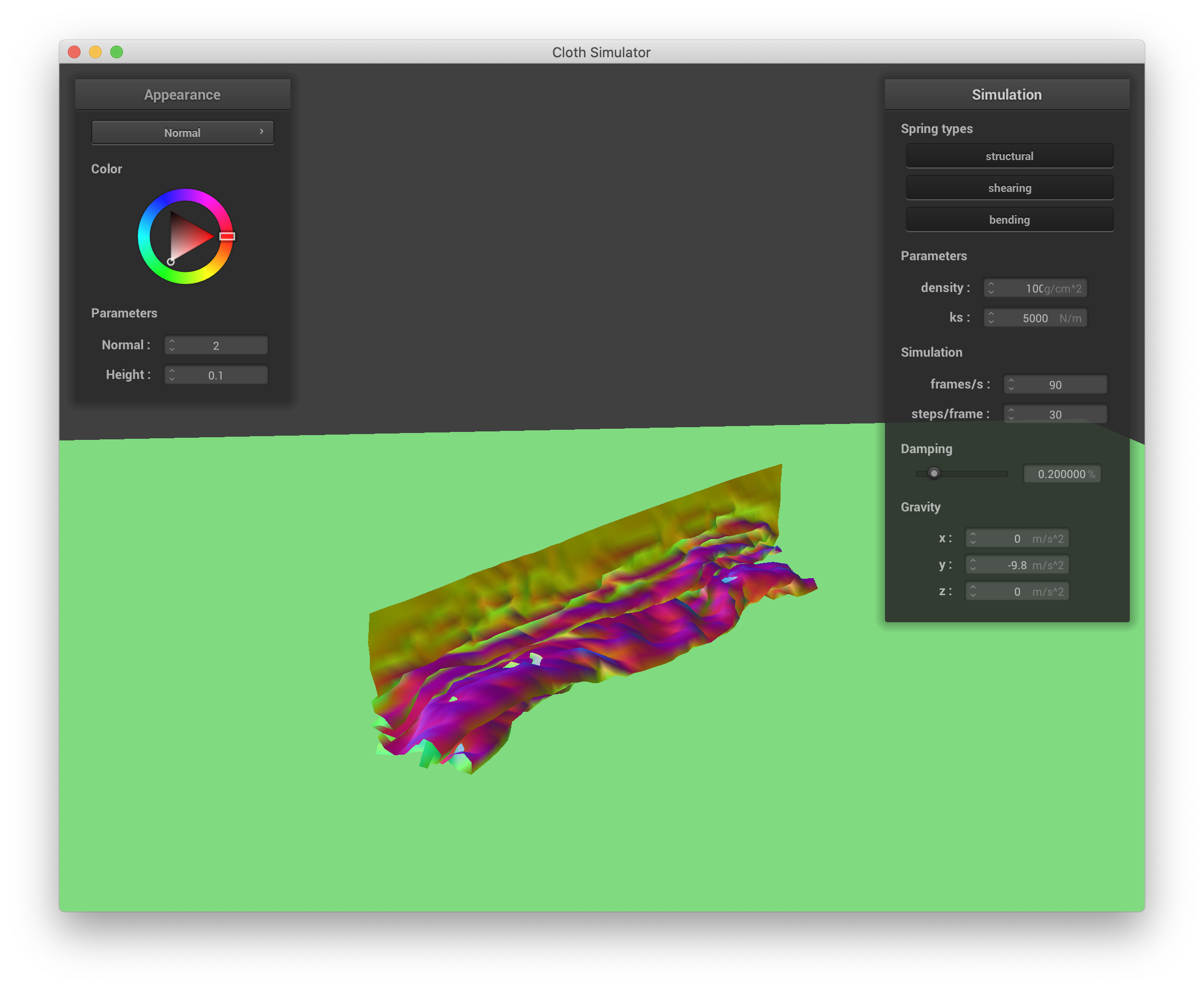
|
|
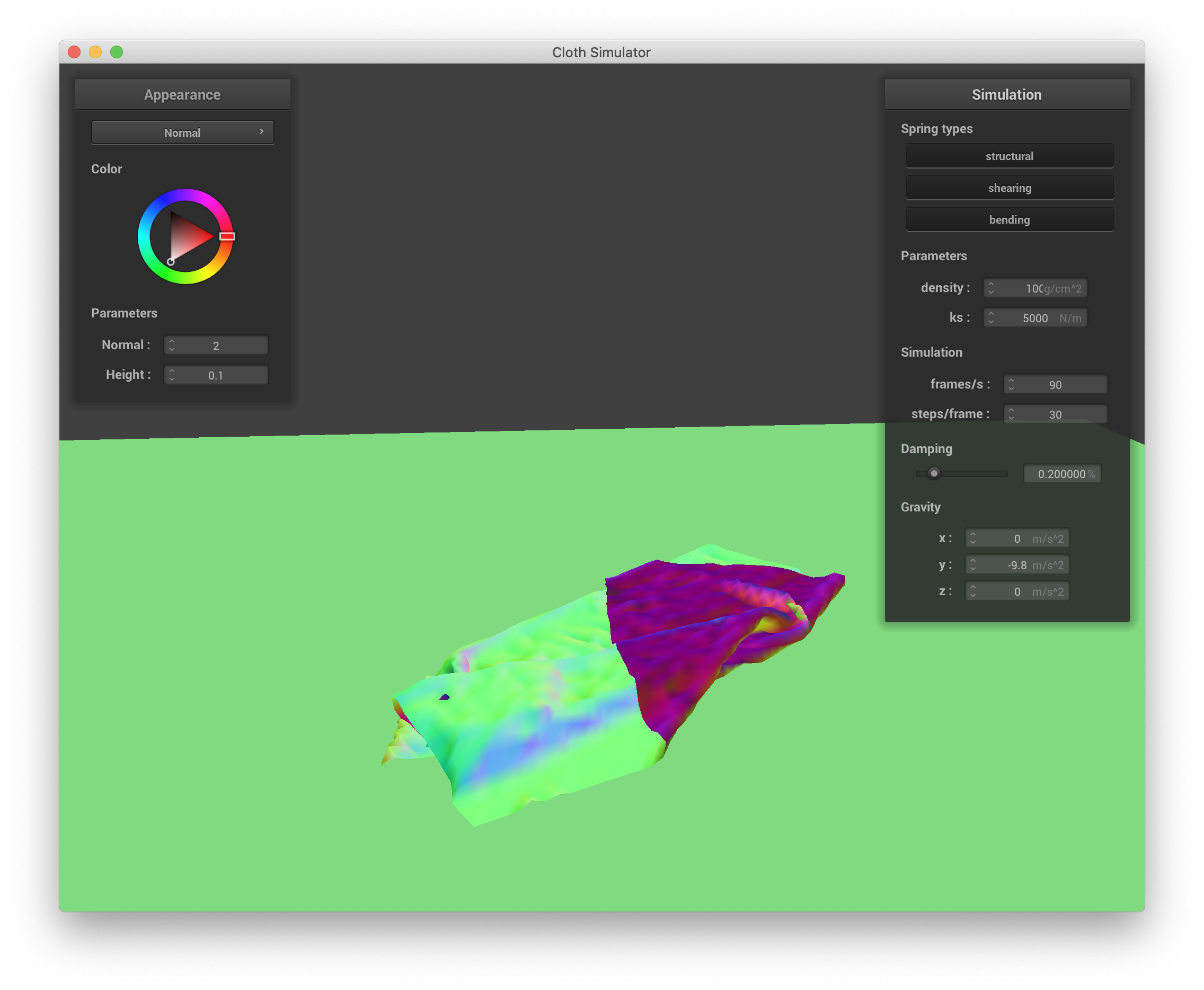
Varying the spring constant also changes how the cloth falls and eventually rests. Lowering the spring constant decreases the structural rigidity of the cloth and reuslts in the cloth crumpling very finely upon itself, eventually resting in a rather wrinkled state. Below are screenshots of the simulation with ks = 0.1:
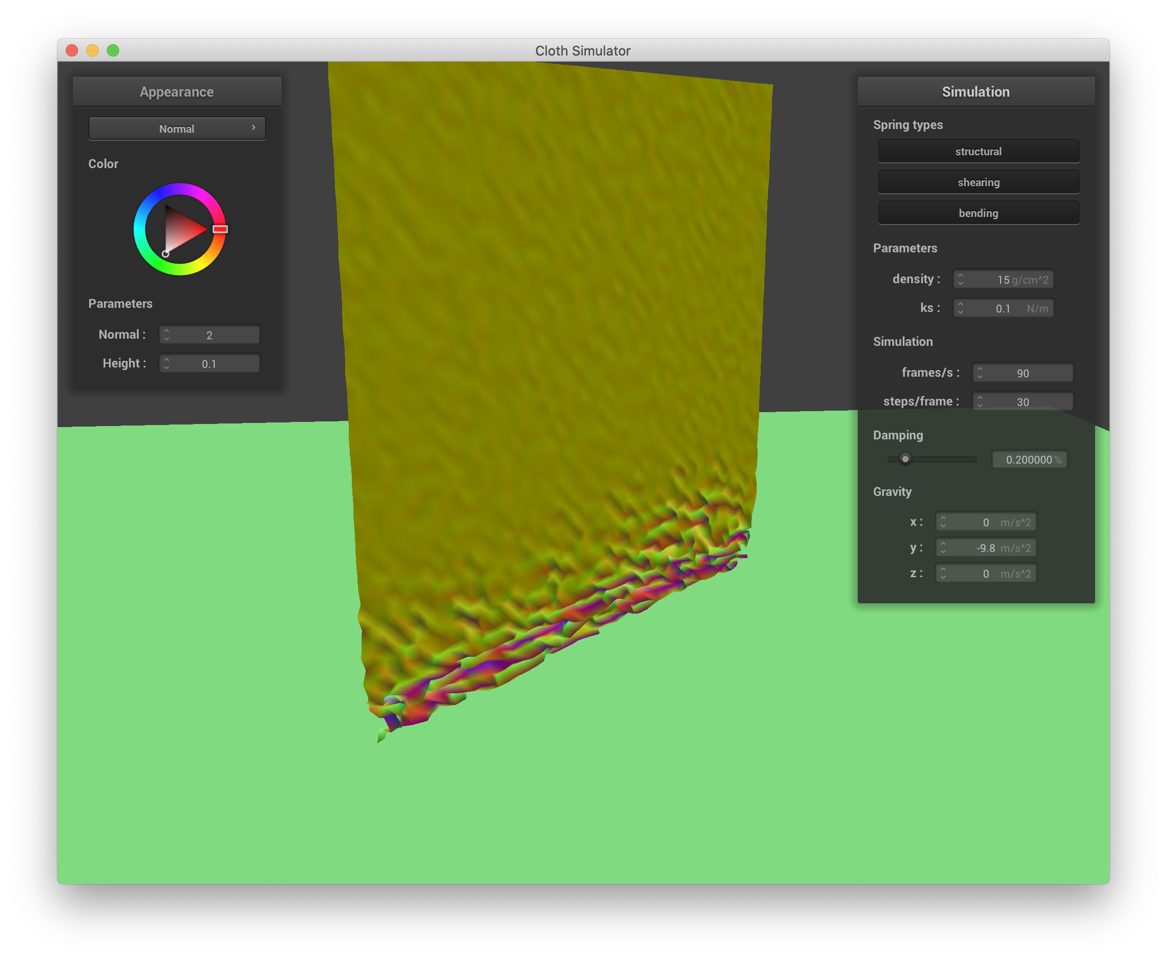
ks = 0.1 N/m |

ks = 0.1 N/m |
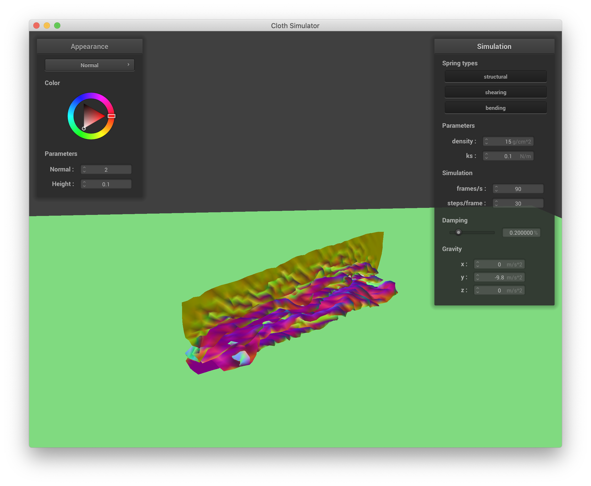
ks = 0.1 N/m |
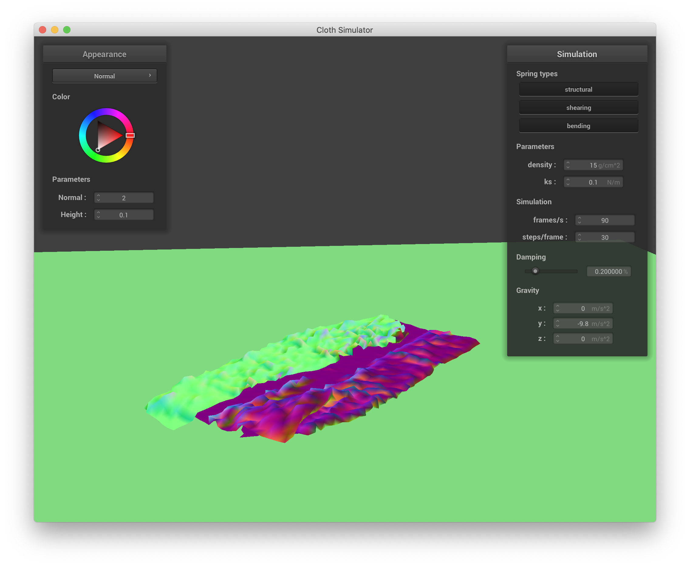
ks = 0.1 N/m |
Conversely, a larger spring constant ks means that the cloth is more stiff and tends to hold its shape as it falls, leading to larger and smoother ruffles as it falls and a smoother final state. Below are screenshots of the simulation with ks = 100000:
ks = 100000 N/m |
ks = 100000 N/m |
ks = 100000 N/m |

ks = 100000 N/m |
Part V: Shaders
In this section, diffuse, Blinn-Phong, texture maping, bump & displacement mapping, and mirror shaders are implemented in GLSL. A shader program is a program that executes once per vertex or fragment to return the color associated with that point, drawing upon the texture associated with that point as well as the desired lighting model. Shaders uses the same underlying principles of calculating color that we explored in ray tracing, except shaders run in parallel to CPU processing on GPU, allowing for fast, real-time textured renderings. A vertex shader processes vertices from the input geometry and provides outputs (e.g. vertex position) for the GPU to render triangles and generate fragments (here, we modify the default vertex shader for displacement mapping only). The fragment shader then draws on data from the vertex shader, as well as other inputs like a texture file, camera position, etc. to determine the color assigned to each pixel.
A diffuse fragment shader is implemented in shaders/Diffuse.frag using the simple formula for diffuse lighting from lecture of out_color = kd * u_light_intensity / r^2 * max(0, v_normal ⋅ l), where r is the distance from the v_position to the light, l is the normalized vector pointing from v_position to the light, and all vec4 types are truncated to 3D coordinates with .xyz. I used a diffuse coefficient factor of kd = 1.0. Below is a screenshot from sphere.json with diffuse shading:
sphere.json, diffuse shading |
The Blinn-Phong shading model improves upon the diffuse-only shading model and takes into account ambient lighting (uniform regardless of the objects in the scene), diffuse lighting, and specular lighting to deliver rendering that includes viewing direction-dependent specular highlights, leading to more realistic appearances for objects that have some shine. The specular component in the Blinn-Phong model accounts for partial mirror-like reflections that occur even when the vector of reflection between the ray to the light source and the ray to the camera (i.e. the half-angle) isn't quite aligned with the surface normal, manifesting as spatially-local highlights. Blinn-Phong fragment shading is implemented in shaders/Phong.frag by adding the ambient (ka * Ia), diffuse (as above), and specular (ks * I/r^2 * max(0, n ⋅ h)^p) components together. A couple of issues I had here were that I was forgetting to normalize some vectors in the process, and that the constants I had picked were so far off that I wasn't getting specular effects like I expected. In the end, I chose ka * Ia = (0.2, 0.2, 0.2), kd = 0.8, ks = 0.5, and p = 40. Below are screenshots showing the ambient, diffuse, and specular outputs separately:
|
|
|
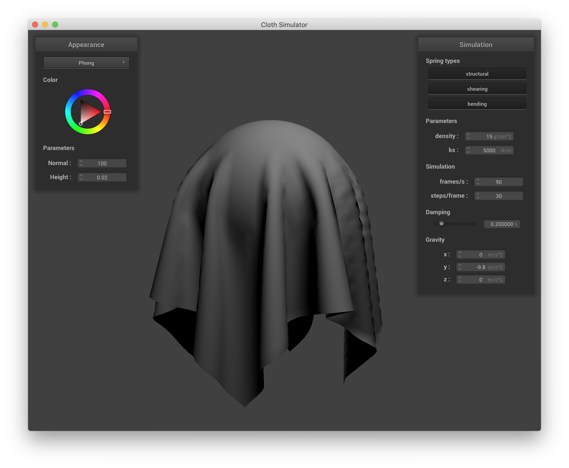
Below is a screenshot from sphere.json using the entire Blinn-Phong shading model:

sphere.json, Blinn-Phong shading |
A texture mapping fragment shader is implemented in shaders/Texture.frag simply by setting the output color to the result of calling texture() on the input sampler texture file and input uv, v_uv. Below is a screenshot from sphere.json with texture mapping using one of my personal photos of a primate as a texture:
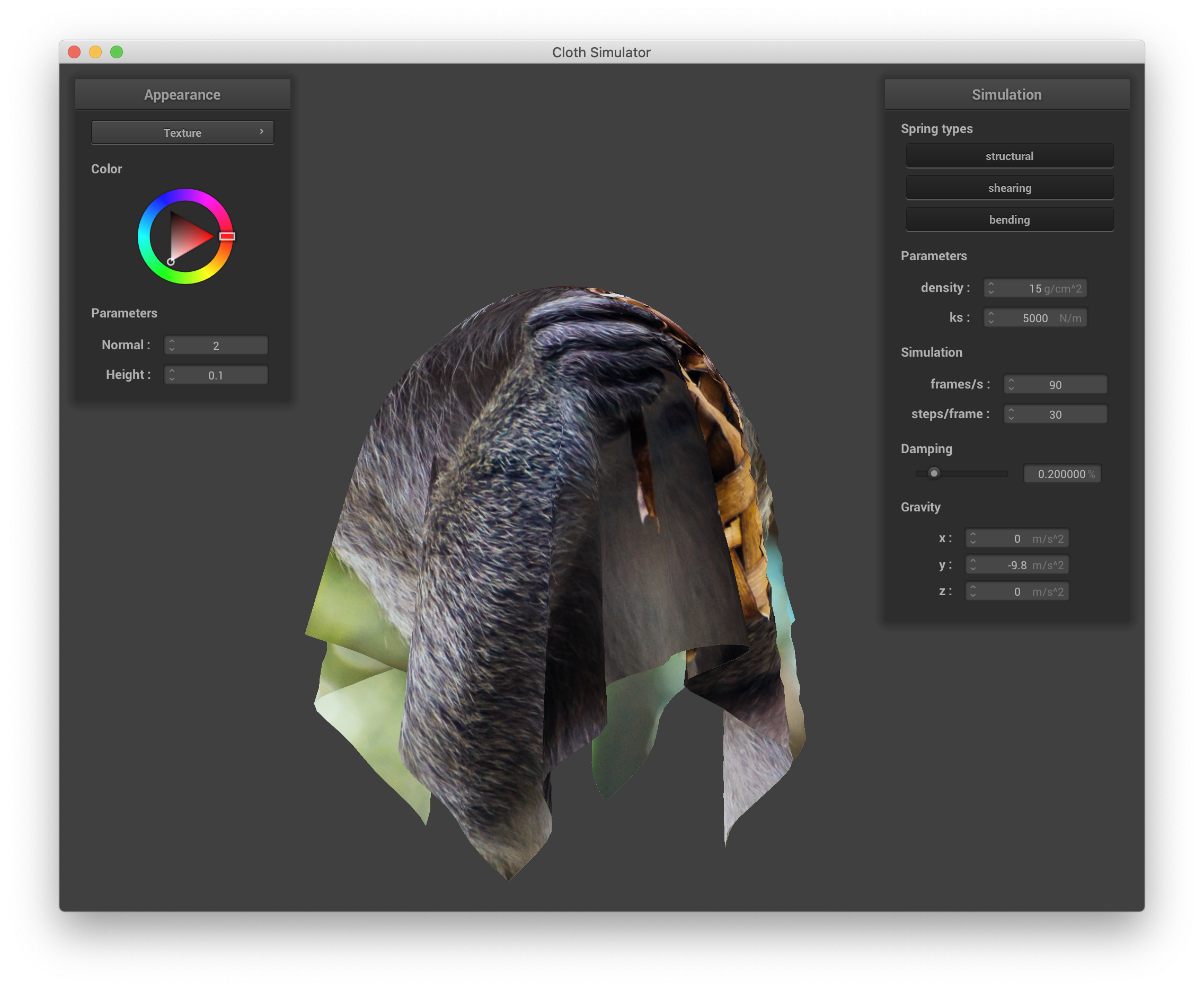
sphere.json, texture mapping |

|
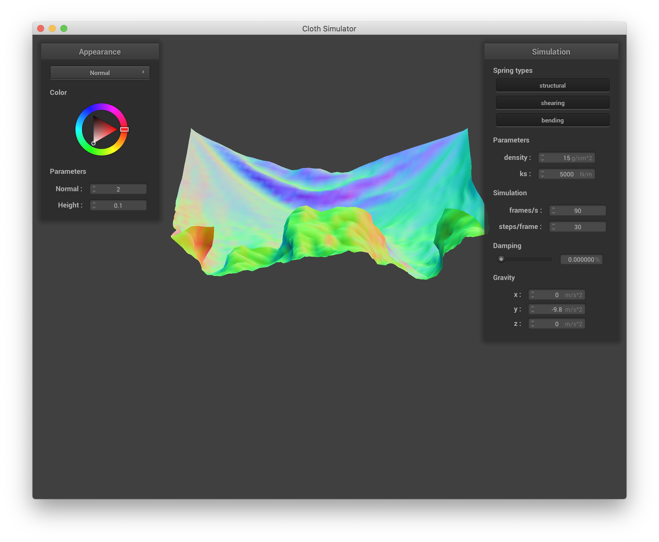
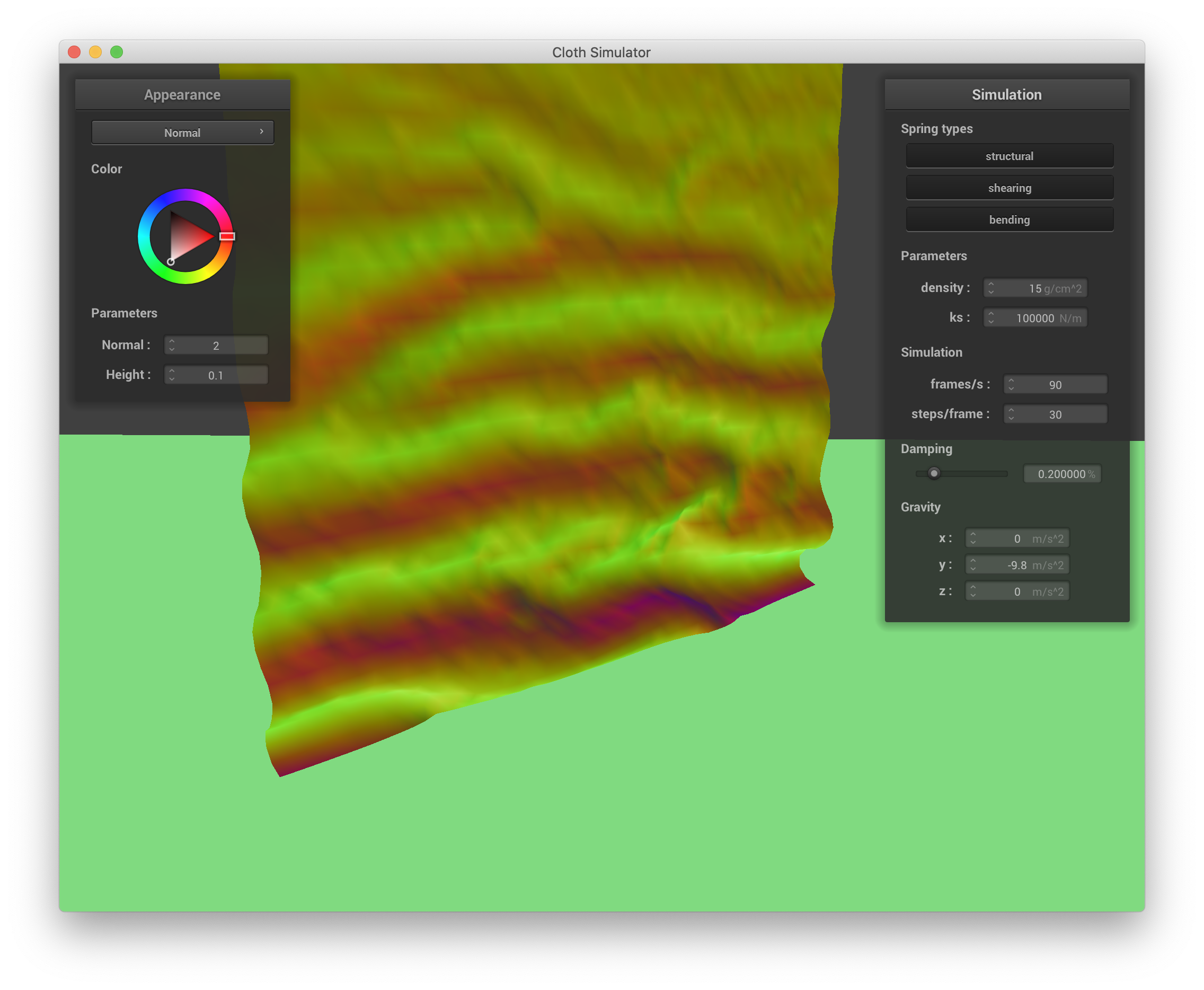
A bump mapping fragment shader is implemented in shaders/Bump.frag by calculating a modified normal vector given the input texture and using that normal vector for Blinn-Phong shading as usual. To calculate the new normal vector, we find the tangent-bitangent normal (TBN) matrix as TBN = [t n x t n], where t is the input tangent vector and n is the input normal vector. We compute the local space normal as n0 = (-dU, -dV, 1), where dU and dV represent height changes when small changes in u or v are made. To calculate these terms, we define a function h(u, v) that returns the height at texture coordinates u and v by returning the r component of texture() given the input texture and uv coordinates v_uv. dU is then (h(u + 1/texture_width, v) - h(u,v)) * kh * kn, and dV = (h(u, v + 1/texture_height) - h(u,v)) * kh * kn, where kh and kn are height and normal scaling factors that are inputs to the shader. Finally, the displaced normal that is used to calculate the Blinn-Phong shading components is nd = TBN * n0. Below is a screenshot from sphere.json with bump mapping. I used texture_3.png as my texture here. The normal and height are set to 100 and 0.02 in the GUI to better match the magnitude of effect seen in the assignment spec. The same parameters from the Blinn-Phong shader as described previously are also used here.
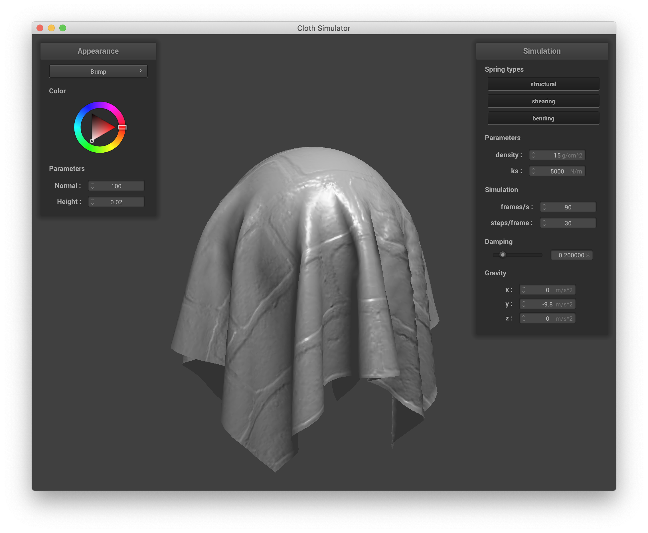
sphere.json, bump mapping |
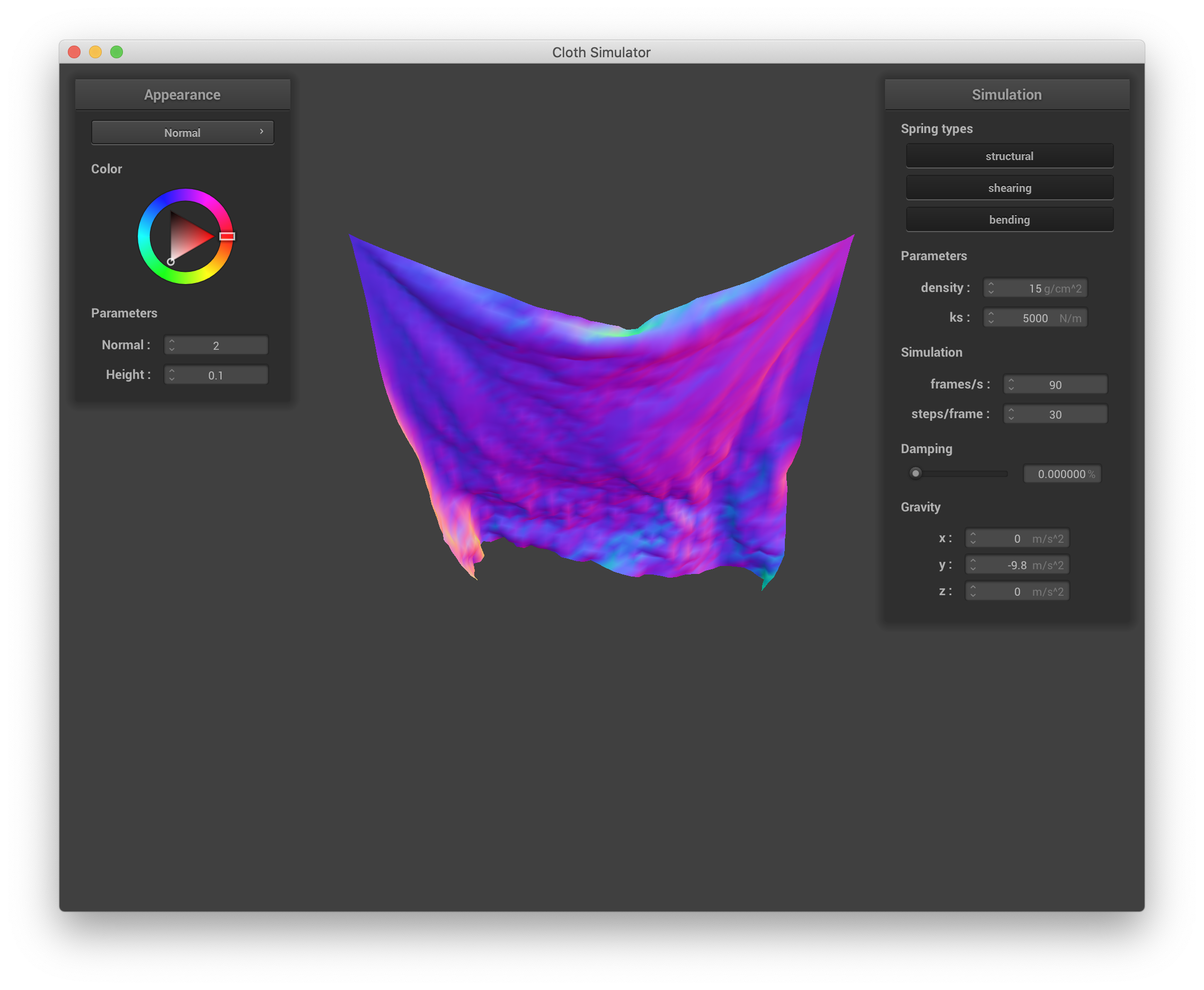
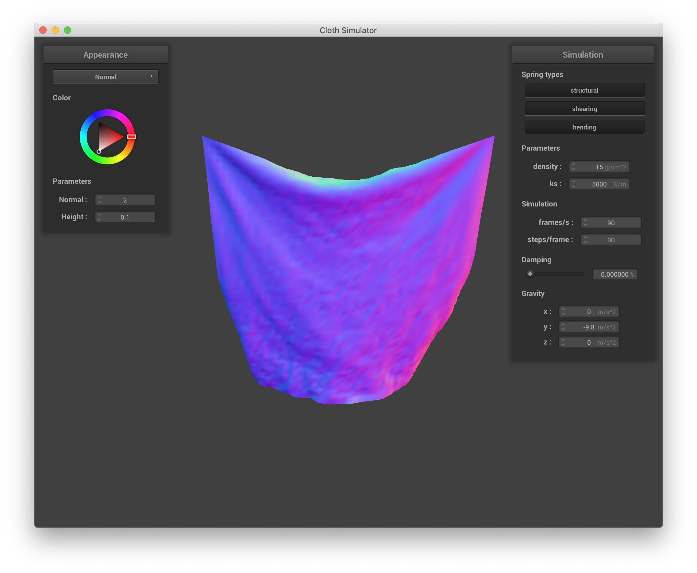
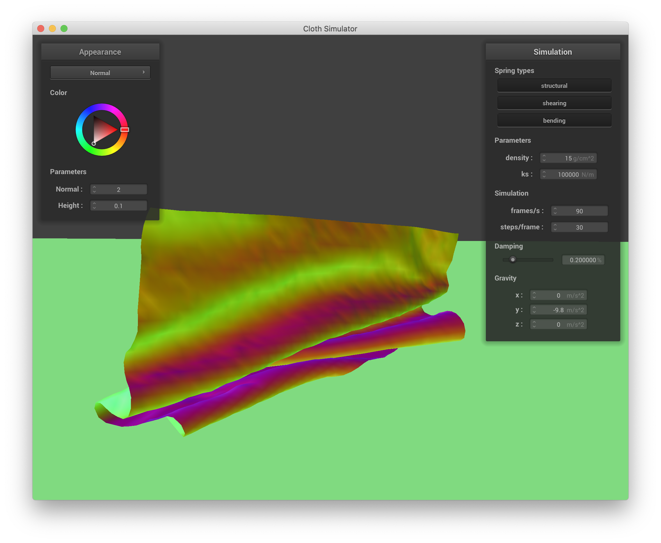
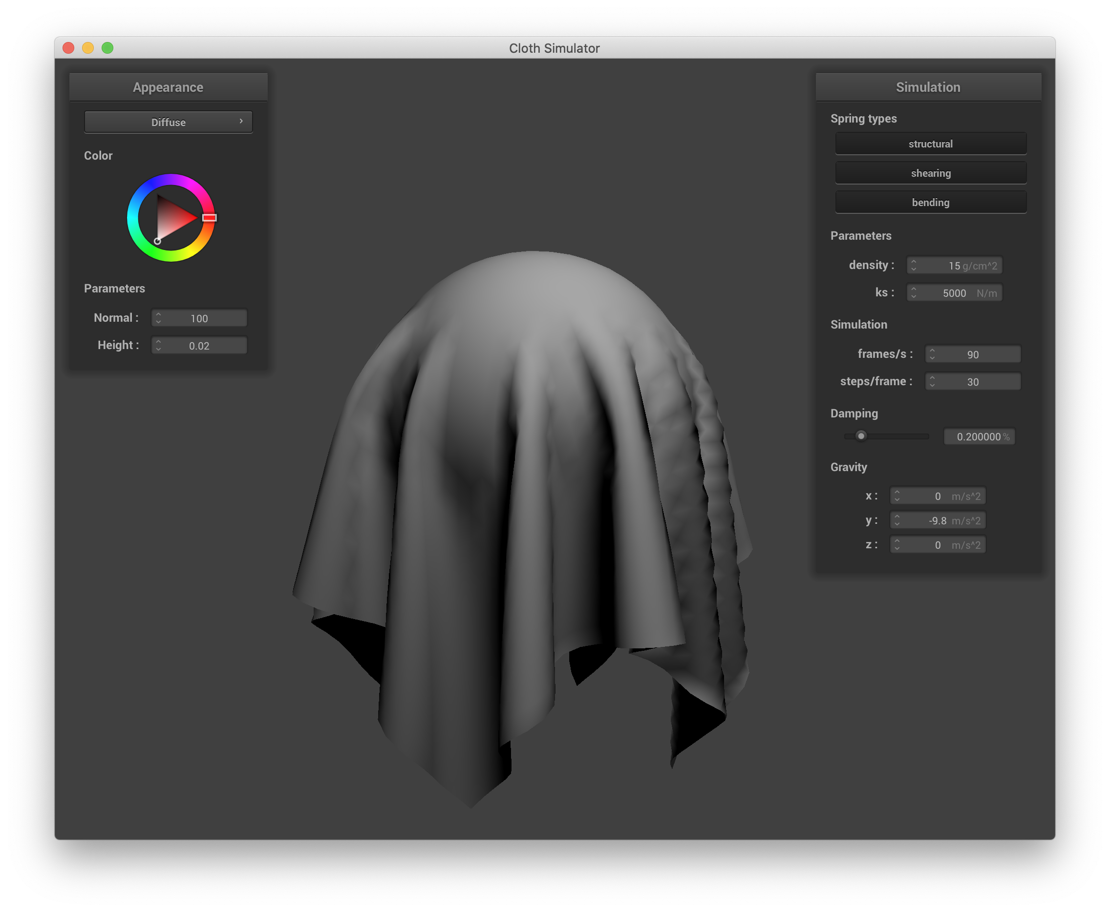
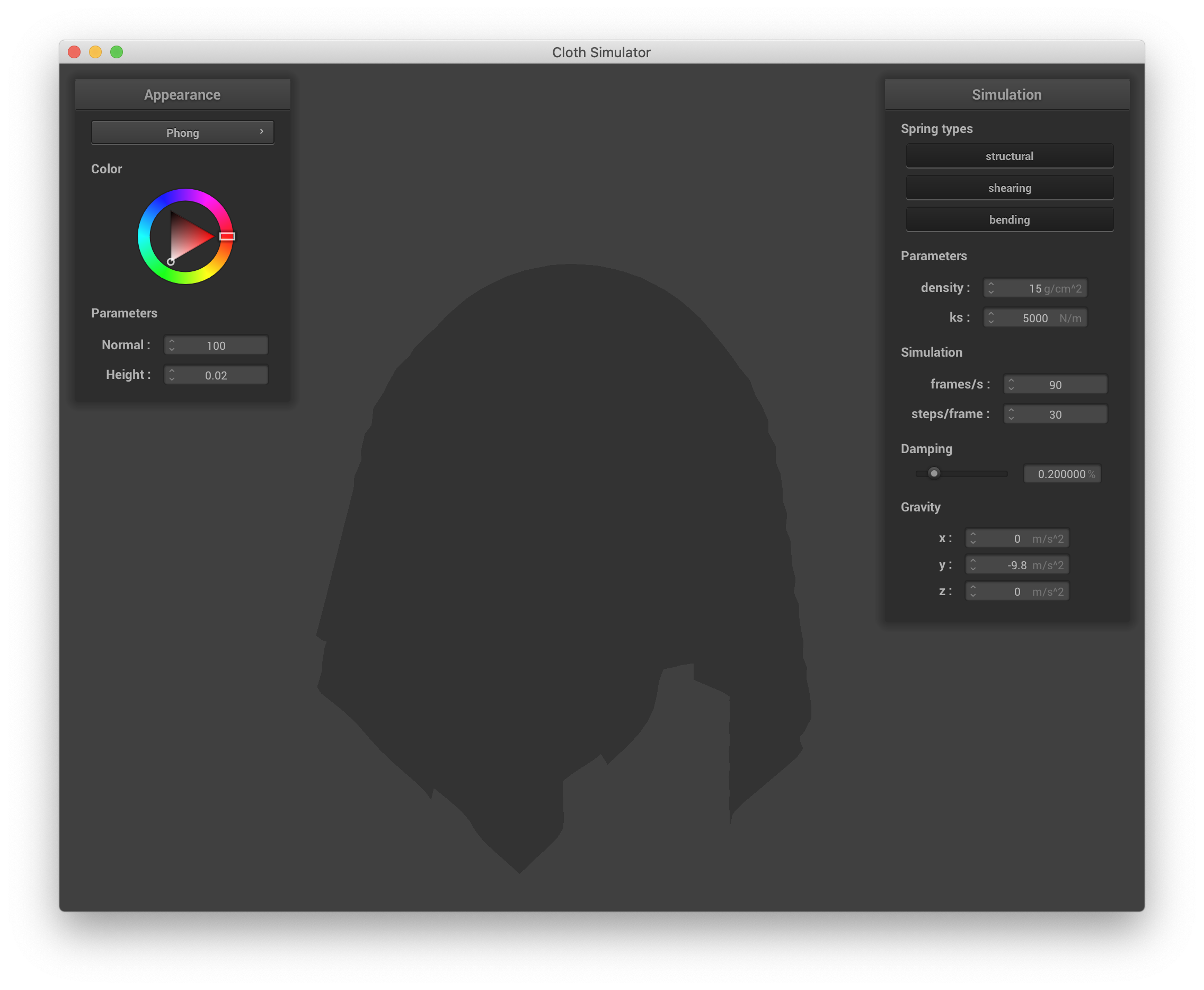
Displacement mapping builds upon bump mapping (the fragment shader shaders/Displacement.frag is a copy of shaders/Bump.frag), except the actual geometry (vertex positions) of the objects are modified to be consistent with the modified shading in the respective vertex shading program. In shaders/Displacement.vert, we simply offset the v_position term by n * h(uv) *kh (where h() is a function as determined in other shaders, n is the normalized vector u_model * the input normal vector, and kh is the height scaling constant as before) before passing it to gl_Position to calculate the vertex's position. Below is a screenshot from sphere.json with displacement mapping. The normal and height are set to 100 and 0.02 in the GUI as before. The same parameters from the Blinn-Phong shader are also used here.
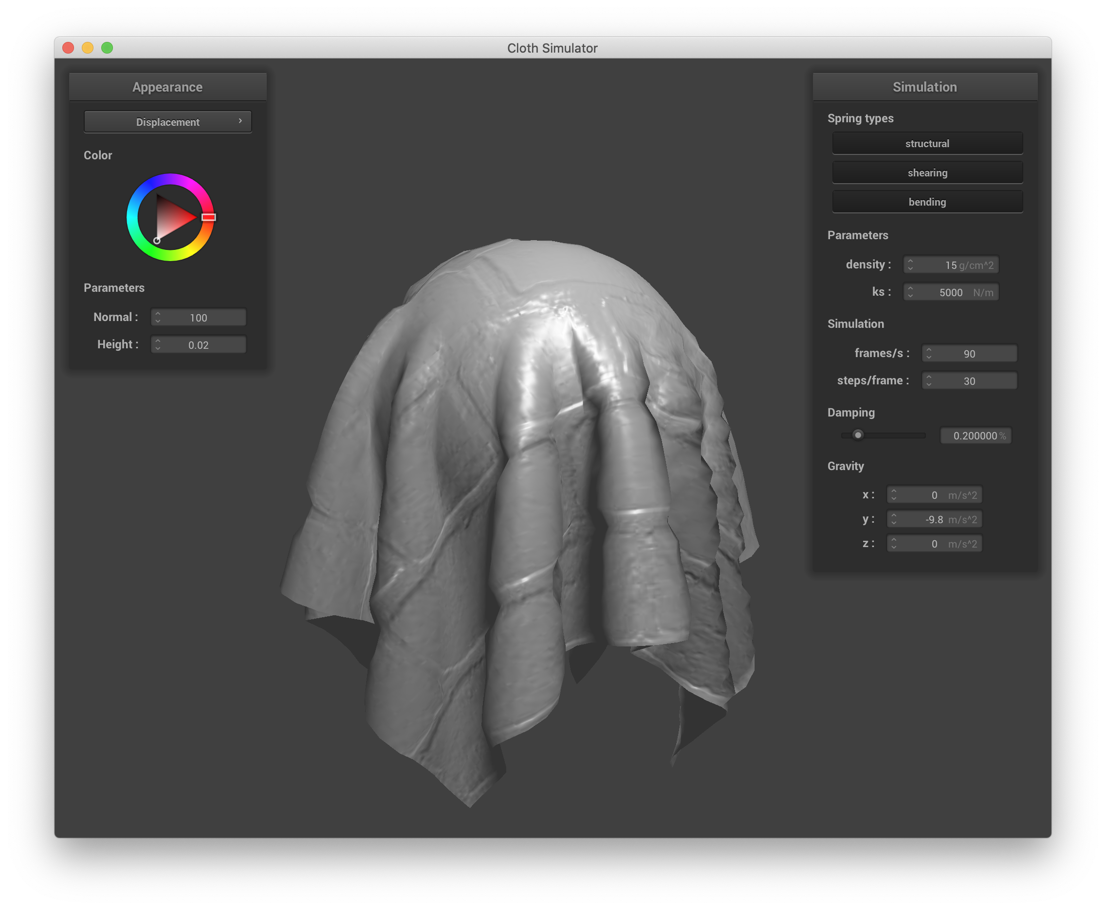
sphere.json, displacement mapping |
Both bump and displacement mapping result in renders that effectively show the applied texture. We can see, however, that while the cloth with bump mapping is still essentially a smooth cloth that is just shaded to look like it has a brick texture, the cloth with displacement mapping actually has the physical ridges and bumps that the texture implies (this is most obvious near the cloth's edges/outline), which is particularly effective for such a texture.
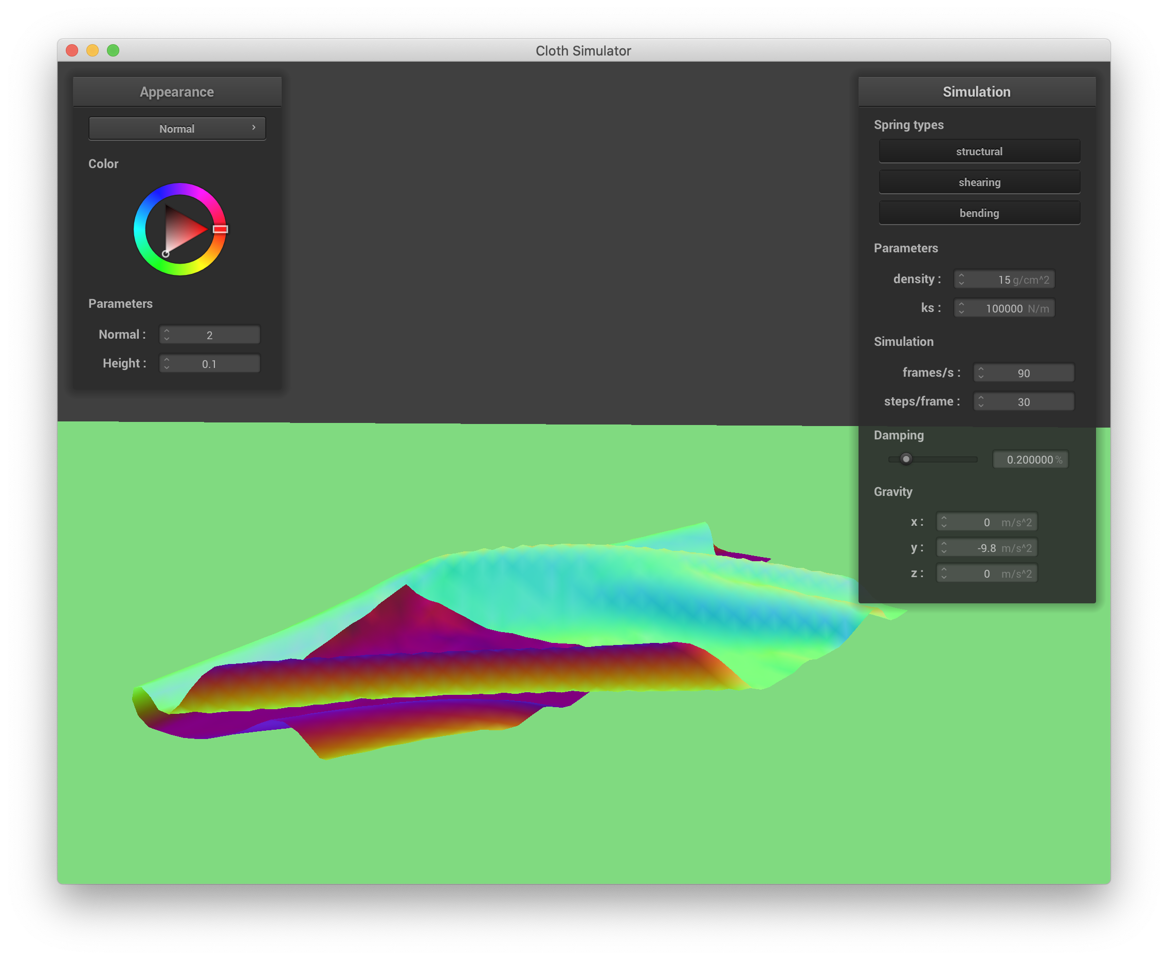
Below are screenshots of just the sphere with bump and displacement mapping shading showing the effect of changing the sphere mesh's coarseness. Bump mapping for this brick texture is basically unaffected, but we can see an obvious difference in the case of displacement mapping. When the sphere's mesh resolution is low (set with -o 16 -a 16), the whole sphere just becomes a little bumpy because the large spacing of its vertices leads to undersampling with respect to the texture, and it is difficult to tell that these bumps correspond to anything in the texture at all. However, when the sphere's resolution is high (set with -o 128 -a 128), the parts of the sphere's mesh that were adjusted to reflect the brick's geometry are very clearly aligned with the underlying grout and ridges in the brick (the grout lines are crisp incut areas), giving a more convincing appearance.

sphere.json, bump mapping w/ 16x16 sphere resolution |
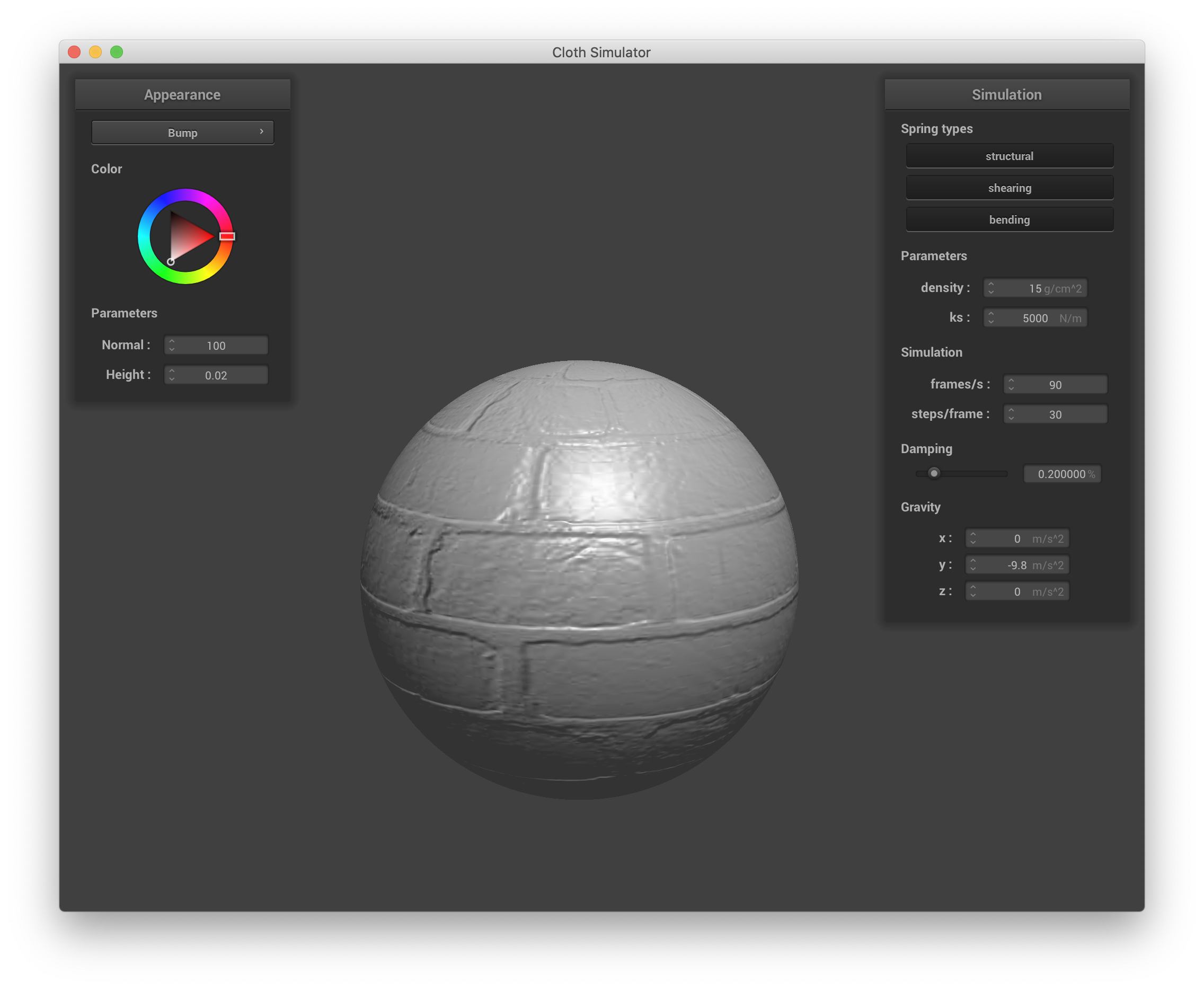
sphere.json, bump mapping w/ 128x128 sphere resolution |

sphere.json, displacement mapping w/ 16x16 sphere resolution |
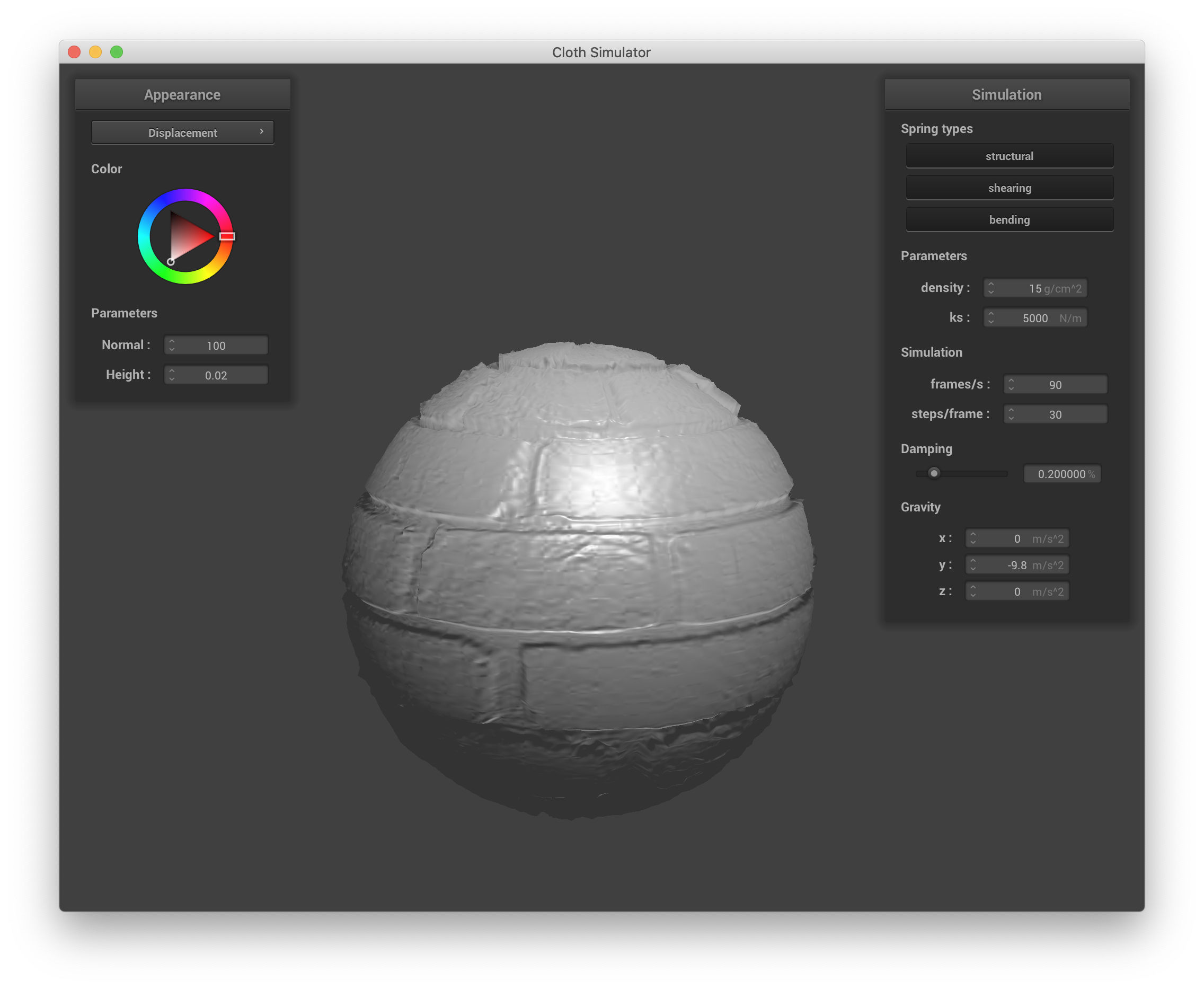
sphere.json, displacement mapping w/ 128x128 sphere resolution |
When the simulation is run and the cloth falls onto these spheres, however, this difference becomes unnoticeable.
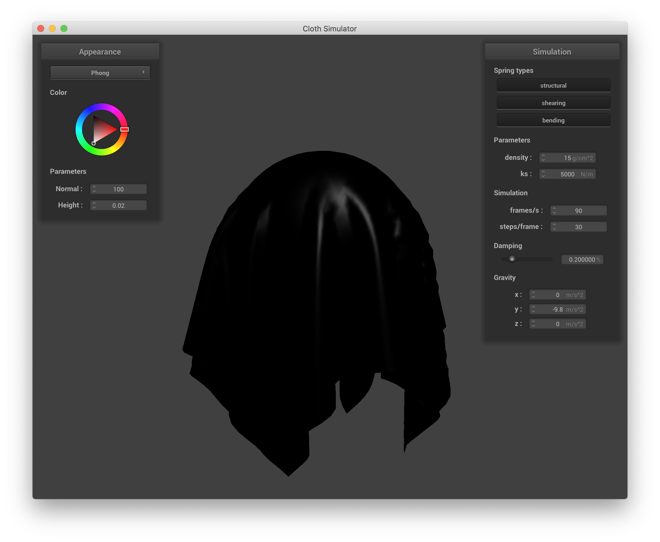
Finally, for environment-mapped reflections, we implement a mirror fragment shader in shaders/Mirror.frag. The outgoing eye-ray direction vector wo is simply the normalized vector from the input fragment v_position to the input camera position u_cam_pos. The incoming eye-ray direction vector wi is the reflection of wo across the input surface normal, v_normal. The calculated color is the sampled environment map for the incoming wi, which is just the result of calling texture() on inputs u_texture_cubemap and wi. Below is a screenshot from sphere.json with mirror shading and environment-mapped reflections:

sphere.json, mirror shading |